Advanced Calculus of Several Variables (1973)
Part V. Line and Surface Integrals; Differential Forms and Stokes' Theorem
Chapter 7. THE CLASSICAL THEOREMS OF VECTOR ANALYSIS
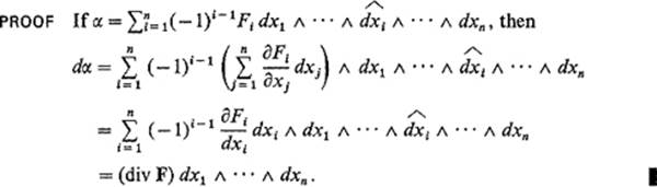
In this section we give the classical vector formulations of certain important special cases of the general Stokes’ theorem of Section 6 . The case n = 3, k = 1 yields the original (classical) form of Stokes’ theorem, while the case n= 3, k = 2 yields the “divergence theorem,” or Gauss' theorem.
If F : ![]() n →
n → ![]() n is a
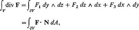
n is a ![]() vector field with component functions F1, . . . , Fn, the divergence of F is the real-valued function div F :
vector field with component functions F1, . . . , Fn, the divergence of F is the real-valued function div F : ![]() n →
n → ![]() defined by
defined by
![]()
The reason for this terminology will be seen in Exercise 7.10. The following result is a restatement of the case k = n − 1 of Stokes' theorem.
Theorem 7.1 Let F be a ![]() vector field defined on a neighborhood of the compact oriented smooth n-manifold-with-boundary
vector field defined on a neighborhood of the compact oriented smooth n-manifold-with-boundary ![]() . Then
. Then
![]()
The divergence theorem in ![]() n is the statement that, if F and V are as in Theorem 7.1 , then
n is the statement that, if F and V are as in Theorem 7.1 , then
![]()
where N is the unit outer normal vector field on ∂V, and ∂V is positively oriented (as the boundary of ![]() ). The following result will enable us to show that the right-hand side of (2) is equal to the right-hand side of (3) .
). The following result will enable us to show that the right-hand side of (2) is equal to the right-hand side of (3) .
Theorem 7.2 Let M be an oriented smooth (n − 1)-manifold in ![]() n with surface area form
n with surface area form
![]()
Then, for each i = 1, . . . , n, the restrictions to each tangent plane of M, of the differential (n − 1)-forms
![]()
are equal.
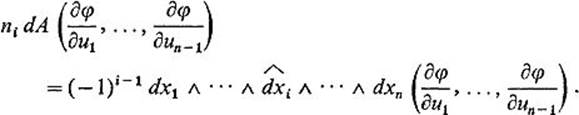
That is, if the vectors v1, . . . , vn−1 are tangent to M at some point x, then
![]()
For brevity we write
![]()
remembering that we are only asserting the equality of the values of these two differential (n − 1)-forms on (n − 1)-tuples of tangent vectors to M.
PROOF Let v1, . . . , vn−1 be tangent vectors to M at the point ![]() , and let φ : U → M be an orientation-preserving coordinate patch with
, and let φ : U → M be an orientation-preserving coordinate patch with ![]() . Since the vectors
. Since the vectors
![]()
constitute a basis for the tangent plane to M at x, there exists an (n − 1) × (n − 1) matrix A = (aij) such that
![]()
If α is any (n − 1)-multilinear function on ![]() n, then
n, then
![]()
by Exercise 5.15 . It therefore suffices to show that
We have seen in Exercise 5.13 that
where
![]()
Consequently
as desired.
![]()
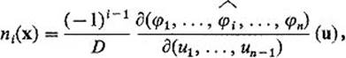
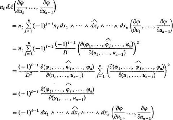
In our applications of this theorem, the following interpretation, of the coefficient functions ni of the surface area form
![]()
of the oriented (n −1)-manifold M, will be important. If M is the positively-oriented boundary of the compact oriented n-manifold-with-boundary ![]() , then the ni are simply the components of the unit outer normal vector field Non M = ∂V (see Exercise 6.7) .
, then the ni are simply the components of the unit outer normal vector field Non M = ∂V (see Exercise 6.7) .
Example 1 We consider the case n = 3. If V is a compact 3-manifold-with-boundary in ![]() 3, and N = (n1, n2, n3) is the unit outer normal vector field on ∂V, then the surface area form of ∂V is
3, and N = (n1, n2, n3) is the unit outer normal vector field on ∂V, then the surface area form of ∂V is
![]()
and Eq. (4) yields
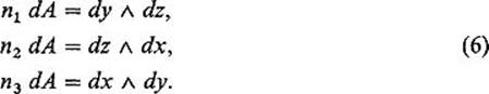
Now let F = (F1, F2, F3) be a ![]() vector field in a neighborhood of V. Then Eqs. (6) give
vector field in a neighborhood of V. Then Eqs. (6) give
![]()
so
![]()
Upon combining this equation with Theorem 7.1 , we obtain
the divergence theorem in dimension 3. Equation (7) , which in essence expresses an arbitrary 2-form on ∂V as a multiple of ∂A, is frequently used in applications of the divergence theorem.
The divergence theorem is often applied to compute a given surface integral by “transforming” it into the corresponding volume integral. The point is that volume integrals are usually easier to compute than surface integrals. The following two examples illustrate this.
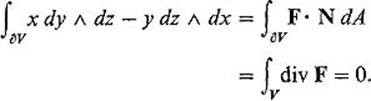
Example 2 To compute ∫∂v x dy ![]() dz − y dz
dz − y dz ![]() dx, we take F = (x, − y, 0). Then div F ≡ 0, so
dx, we take F = (x, − y, 0). Then div F ≡ 0, so
Example 3 To compute ![]() , take F = (0, y, xz). Then div F = 1 + x, so
, take F = (0, y, xz). Then div F = 1 + x, so
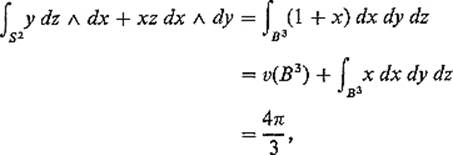
since the last integral is obviously zero by symmetry.
Example 4 Let S1 and S2 be two spheres centered at the origin in ![]() 3 with S1 interior to S2, and denote by R the region between them. Suppose that F is a vector field such that div F = 0 at each point of R. If N0 is the outer normal vector field on ∂R (pointing outward at each point of S2, and inward at each point of S1, as in Fig. 5.42) , then the divergence theorem gives
3 with S1 interior to S2, and denote by R the region between them. Suppose that F is a vector field such that div F = 0 at each point of R. If N0 is the outer normal vector field on ∂R (pointing outward at each point of S2, and inward at each point of S1, as in Fig. 5.42) , then the divergence theorem gives
![]()
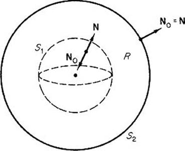
Figure 5.42
If N denotes the outer normal on both spheres (considering each as the positively oriented boundary of a ball), then N = N0 on S2, while N = − N0 on S1. Therefore
![]()
so we conclude that
![]()
The proof of the n-dimensional divergence theorem is simply a direct generalization of the proof in Example 1 of the 3-dimensional divergence theorem.
Theorem 7.3 If F is a ![]() vector field defined on a neighborhood of the compact n-manifold-with-boundary
vector field defined on a neighborhood of the compact n-manifold-with-boundary ![]() , then
, then
![]()
where N and dA are the outer normal and surface area form of the positively-oriented boundary ∂V.
PROOF In computing the right-hand integral, the (n − 1)-form F · N dA is applied only to (n − 1)-tuples of tangent vectors to ∂V. Therefore we can apply Theorem 7.2 to obtain
Thus Eq. (3) follows immediately from Theorem 7.1.
![]()
The integral ∫∂v F · N dA is sometimes called the flux of the vector field F across the surface ∂V. This terminology is motivated by the following physical interpretation. Suppose that F = ρv, where v is the velocity vector field of a fluid which is flowing throughout an open set containing V, and ρ is its density distribution function (both functions of x, y, z, and t). We want to show that ∫∂v F · N dA is the rate at which mass is leaving the region V, that is, that
![]()
where
![]()
is the total mass of the fluid in V at time T. Let {A1, . . . , Ak} be an oriented paving of the oriented (n − 1)-manifold ∂V, with the (n − 1)-cells A1, . . . , Ak so small that each is approximately an (n − 1)-dimensional parallelepiped (Fig. 5.43) . Let Ni, vi, ρi, and Fi = ρi vi be the values of N, v, ρ, and F at a selected point of Ai. Then the volume of that fluid which leaves the region V through the cell Ai, during the short time interval δt, is approximately equal to the volume of an n-dimensional parallelepiped with base Ai and height (vi δt) · Ni, and the density of this portion of the fluid is approximately ρi. Therefore, if δM denotes the change in the mass of the fluid within V during the time interval δt, then
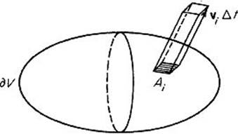
Figure 5.43
Taking the limit as δt → 0, we conclude that
![]()
as desired.
We can now apply the divergence theorem to obtain
![]()
On the other hand, if ∂ρ/∂t is continuous, then by differentiation under the integral sign we obtain
![]()
Consequently
![]()
Since this must be true for any region V within the fluid flow, we conclude by the usual continuity argument that
![]()
This is the equation of continuity for fluid flow. Notice that, for an incompressible fluid (one for which ρ = constant), it reduces to
![]()
We now turn our attention to the special case n = 3, k = 1 which, as we shall see, leads to the following classical formulation of Stokes' theorem in ![]() 3:
3:
![]()
where D is an oriented compact 2-manifold-with-boundary in ![]() 3, N and T are the appropriate unit normal and unit tangent vector fields on D and ∂D, respectively, F = (F1, F2, F3) is a
3, N and T are the appropriate unit normal and unit tangent vector fields on D and ∂D, respectively, F = (F1, F2, F3) is a ![]() vector field, and curl F is the vector field defined by
vector field, and curl F is the vector field defined by
![]()
This definition of curl F can be remembered in the form
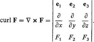
That is, curl F is the result of formal expansion, along its first row, of the 3 × 3 determinant obtained by regarding curl F as the cross product of the gradient operator δ = (∂/∂x, ∂/∂y, ∂/∂z) and the vector F.
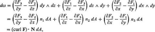
If ω = F1 dx + F2 dy + F3 dz is the differential 1-form whose coefficient functions are the components of F, then
![]()
by Example 2 of Section 5 . Notice that the coefficient functions of the 2-form dω are the components of the vector curl F. This correspondence, between ω and F on the one hand, and between dω and curl F on the other, is the key to the vector interpretation of Stokes' theorem.
The unit normal N and unit tangent T, in formula (8) above, are defined as follows. The oriented compact 2-manifold-with-boundary D is (by definition) a subset of an oriented smooth 2-manifold ![]() . The orientation of Mprescribes a unit normal vector field N on M as in Exercise 5.13 . Specifically,
. The orientation of Mprescribes a unit normal vector field N on M as in Exercise 5.13 . Specifically,
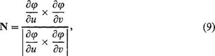
where φ is an orientation-preserving coordinate patch on M. If n is the outer normal vector field on ∂D—that is, at each point of ∂D, n is the tangent vector to M which points out of D (Fig. 5.44) —then we define the unit tangent on ∂D by
![]()
The reader may check “visually” that this definition of T yields the same orientation of ∂D as in the statement of Green's theorem, in case D is a plane region. That is, if one proceeds around ∂D in the direction prescribed by T,remaining upright (regarding the direction of N as “up”), then the region D remains on his left.
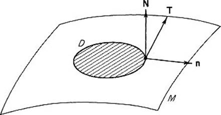
Figure 5.44
Theorem 7.4 Let D be an oriented compact 2-manifold-with-boundary in ![]() 3, and let N and T be the unit normal and unit tangent vector fields, on D and ∂D, respectively, defined above. If F is a
3, and let N and T be the unit normal and unit tangent vector fields, on D and ∂D, respectively, defined above. If F is a ![]() vector field on an open set containing D, then
vector field on an open set containing D, then
![]()
PROOF The orientation of ∂D prescribed by (10) is the positive orientation of ∂D, as defined in Section 6. If
![]()
it follows that
![]()
See Exercise 1.21 or the last paragraph of Section 1 .
Applying Theorem 7.2 in the form of Eq. (6) , we obtain
so
![]()
Since ∫D dω = ∫∂D ω by the general Stokes' theorem, Eqs. (11) and (12) imply Eq. (8) .
![]()
Stokes' Theorem is frequently applied to evaluate a given line integral, by “transforming” it to a surface integral whose computation is simpler.
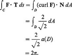
Example 5 Let F(x, y, z) = (x, x + y, x + y + z), and denote by C the ellipse in which the plane z = y intersects the cylinder x2 + y2 = 1, oriented counterclockwise around the cylinder. We wish to compute ∫c F · T ds. Let D be the elliptical disk bounded by C. The semiaxes of D are 1 and ![]() , so
, so ![]() . Its unit normal is
. Its unit normal is ![]() , and curl F = (1, −1, 1). Therefore
, and curl F = (1, −1, 1). Therefore
Another typical application of Stokes' theorem is to the computation of a given surface integral by “replacing” it with a simpler surface integral. The following example illustrates this.
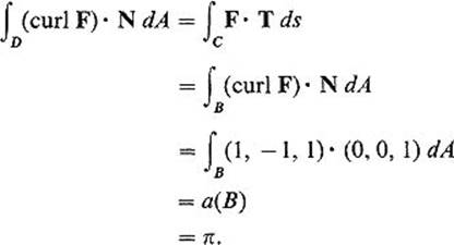
Example 6 Let F be the vector field of Example 5 , and let D be the upper hemisphere of the unit sphere S2. We wish to compute ∫D(curl F) · N dA. Let B be the unit disk in the xy-plane, and C = ∂D = ∂B, oriented counterclockwise. Then two applications of Stokes' theorem give
We have interpreted the divergence vector in terms of fluid flow; the curl vector also admits such an interpretation. Let F be the velocity vector field of an incompressible fluid flow. Then the integral
![]()
is called the circulation of the field F around the oriented closed curve C. If Cr is the boundary of a small disk Dr of radius r, centered at the point p and normal to the unit vector b (Fig. 5.45) , then
![]()
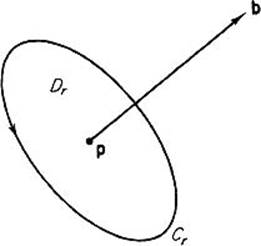
Figure 5.45
Taking the limit as r → 0, we see that
![]()
Thus the b-component of curl F measures the circulation (or rotation) of the fluid around the vector b. For this reason the fluid flow is called irrotational if curl F = 0.
For convenience we have restricted our attention in this section to smooth manifolds-with-boundary. However the divergence theorem and the classical Stokes' theorem hold for more general regions. For example, if V is an oriented cellulated n-dimensional region in ![]() n, and F is a
n, and F is a ![]() vector field, then
vector field, then
![]()
(just as in Theorem 7.3), with the following definition of the surface integral on the right. Let ![]() be an oriented cellulation of V, and let A1, . . . , Ap be the boundary (n − 1)-cells of
be an oriented cellulation of V, and let A1, . . . , Ap be the boundary (n − 1)-cells of ![]() , so
, so ![]() . Let Ai be oriented in such a way that the procedure of Exercise 5.13 gives the outer normal vector field on Ai, and denote by Ni this outer normal on Ai. Then we define
. Let Ai be oriented in such a way that the procedure of Exercise 5.13 gives the outer normal vector field on Ai, and denote by Ni this outer normal on Ai. Then we define
![]()
We will omit the details, but this more general divergence theorem could be established by the method of proof of the general Stokes' theorem in Section 6—first prove the divergence theorem for an oriented n-cell in ![]() n, and then piece together the n-cells of an oriented cellulation.
n, and then piece together the n-cells of an oriented cellulation.
Example 7 Let V be the solid cylinder ![]() . Denote by D0 and D1 the bottom and top disks respectively, and by R the cylindrical surface (Fig. 5.46). Then the outer normal is given by
. Denote by D0 and D1 the bottom and top disks respectively, and by R the cylindrical surface (Fig. 5.46). Then the outer normal is given by
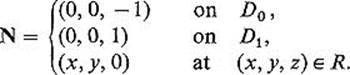
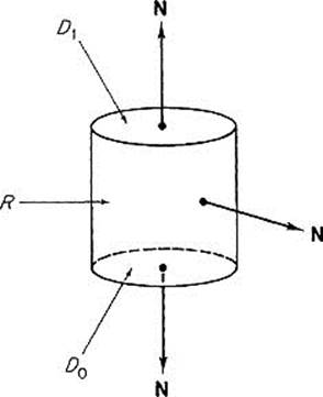
Figure 5.46
If F = (x, y, z), then
Alternatively, we can apply the divergence theorem to obtain
![]()
Similarly, Stokes' theorem holds for piecewise smooth compact oriented surfaces in ![]() 3. A piecewise smooth compact oriented surface S in
3. A piecewise smooth compact oriented surface S in ![]() 3 is the union of a collection {A1, . . . , Ap} of oriented 2-cells in
3 is the union of a collection {A1, . . . , Ap} of oriented 2-cells in ![]() 3, satisfying conditions (b), (c), (d) in the definition of an oriented cellulation (Section 6), with the union ∂S of the boundary edges of these oriented 2-cells being a finite number of oriented closed curves. If F is a
3, satisfying conditions (b), (c), (d) in the definition of an oriented cellulation (Section 6), with the union ∂S of the boundary edges of these oriented 2-cells being a finite number of oriented closed curves. If F is a ![]() vector field, then
vector field, then
![]()
(just as in Theorem 7.4), with the obvious definition of these integrals (as in the above discussion of the divergence theorem for cellulated regions). For example, Stokes' theorem holds for a compact oriented polyhedral surface (one which consists of a nonoverlapping triangles).
Exercises
7.1The moment of inertia I of the region ![]() about the z-axis is defined by
about the z-axis is defined by
![]()
Show that
![]()
7.2Let ρ = (x2 + y2 + z2)1/2.
(a)If F(x, y, z) = ρ · (x, y, z), show that div F = 4ρ. Use this fact and the divergence theorem to show that
![]()
(Ba3 being the ball of radius a) by converting to a surface integral that can be evaluated by inspection.
(b)If F = ρ2 · (x, y, z), compute the integral ![]() div F in a similar manner.
div F in a similar manner.
7.3Find a function g(ρ) such that, if F(x, y, z) = g(ρ)(x, y, z), then div ![]() . Use it to prove that
. Use it to prove that
![]()
if V is a compact 3-manifold-with-boundary in ![]() 3. For example, show that
3. For example, show that
![]()
7.4In each of the following, let C be the curve of intersection of the cylinder x2 + y2 = 1 and the given surface z = f(x, y), oriented counterclockwise around the cylinder. Use Stokes' theorem to compute the line integral by first converting it to a surface integral.
(a)![]()
(b)![]()
(c)![]()
7.5Let the 2-form α be defined on ![]() 3 − p, p = (a, b, c), by
3 − p, p = (a, b, c), by
![]()
(a)Show that dα = 0.
(b)Conclude that ∫M α = 0 if M is a compact smooth 2-manifold not enclosing the point p.
(c)Show that ∫M α = 4π if M is a sphere centered at p.
(d)Show that ∫M α = 4π if M is any compact positively oriented smooth 2-manifold enclosing the point p.
7.6The potential φ(x, y, z) at x = (x, y, z) due to a collection of charges q1, . . . , qm at the points p1, . . . , pm is
![]()
where ri = ![]() x − pi
x − pi![]() . If E = −
. If E = −![]() φ, the electric field vector, apply the previous problem to show that
φ, the electric field vector, apply the previous problem to show that
![]()
if M is a smooth 2-manifold enclosing these charges. This is Gauss' law.
7.7Let f and g be ![]() functions on an open set containing the compact n-manifold-with-boundary
functions on an open set containing the compact n-manifold-with-boundary ![]() , and let N be the unit outer normal on ∂V. The Laplacian
, and let N be the unit outer normal on ∂V. The Laplacian ![]() 2f and the normal derivative ∂f/∂n are defined by
2f and the normal derivative ∂f/∂n are defined by
![]()
Prove Green's formulas in ![]() n:
n:
(a)![]()
(b)![]()
Hint: For (a), apply the divergence theorem with F = f![]() g.
g.
7.8Use Green's formulas in ![]() n to generalize Exercises 2.7 and 2.8 to
n to generalize Exercises 2.7 and 2.8 to ![]() n. In particular, if f and g are both harmonic on
n. In particular, if f and g are both harmonic on ![]() and f = g on ∂V, prove that f = g throughout V.
and f = g on ∂V, prove that f = g throughout V.
7.9Let f be a harmonic function on the open set ![]() . If B is an n-dimensional ball in U with center p and radius a, and S = ∂B, prove that
. If B is an n-dimensional ball in U with center p and radius a, and S = ∂B, prove that
![]()
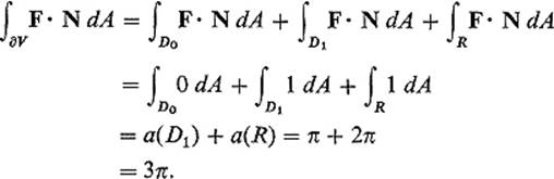
That is, the value of f at the center of the ball B is the average of its values on the boundary S of B. This is the average value property for harmonic functions. Outline: Without loss of generality, we may assume that p is the origin. Define the function g : ![]() n − 0 →
n − 0 → ![]() by
by
![]()
Denote by S![]() a small sphere of radius
a small sphere of radius ![]() > 0 centered at 0, and by V the region between S
> 0 centered at 0, and by V the region between S![]() and S (Fig. 5.47).
and S (Fig. 5.47).
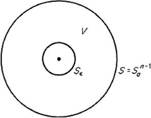
Figure 5.47
(a)Show that g is harmonic, and then apply the second Green's formula (Exercise 7.7) to obtain the formula
![]()
(b)Notice that
![]()
and similarly for the right-hand side of (*), with a replaced by ![]() , because ∂g/∂n = (2 − n)/rn−1. Use the divergence theorem to show that
, because ∂g/∂n = (2 − n)/rn−1. Use the divergence theorem to show that
![]()
so formula (*) reduces to
![]()
(c)Now obtain the average value property for f by taking the limit in (**) as ![]() → 0.
→ 0.
7.10Let F be a ![]() vector field in
vector field in ![]() n. Denote by B
n. Denote by B![]() the ball of radius
the ball of radius ![]() centered at p, and S
centered at p, and S![]() = ∂B
= ∂B![]() . Use the divergence theorem to show that
. Use the divergence theorem to show that
![]()
If we think of F as the velocity vector field of a fluid flow, then this shows that div F(p) is the rate (per unit volume) at which the fluid is “diverging” away from the point p.
7.11Let V be a compact 3-manifold-with-boundary in the lower half-space z < 0 of ![]() 3. Think of V as an object submerged in a fluid of uniform density ρ, its surface at z = 0 (Fig. 5.48). The buoyant force B on V, due to the fluid, is defined by
3. Think of V as an object submerged in a fluid of uniform density ρ, its surface at z = 0 (Fig. 5.48). The buoyant force B on V, due to the fluid, is defined by
![]()
where F = (0, 0, ρz). Use the divergence theorem to show that
![]()
Thus the buoyant force on the object is equal to the weight of the fluid that it displaces (Archimedes).
Figure 5.48
7.12Let U be an open subset of ![]() 3 that is star-shaped with respect to the origin. This means that, if
3 that is star-shaped with respect to the origin. This means that, if ![]() , then U contains the line segment from 0 to p. Let F be a
, then U contains the line segment from 0 to p. Let F be a ![]() vector field on U. Then use Stokes' theorem to prove that curl F = 0 on U if and only if
vector field on U. Then use Stokes' theorem to prove that curl F = 0 on U if and only if
![]()
for every polygonal closed curve C in U. Hint: To show that curl F ≡ 0 implies that the integral vanishes, let C consist of the line segments L1, . . . , Lp. For each i = 1, . . . , p, denote by Ti the triangle whose vertices are the origin and the endpoints of Li. Apply Stokes' theorem to each of these triangles, and then add up the results.