Advanced Calculus of Several Variables (1973)

Part VI. The Calculus of Variations

The calculus of variations deals with a certain class of maximum–minimum problems, which have in common the fact that each of them is associated with a particular sort of integral expression. The simplest example of such a problem is the following. Let f: ³ → be a given function, and denote by the set of all real-valued functions defined on the interval [a, b]. Given , define by

Then F is a real-valued function on . The problem is then to find that element , if any, at which the function attains its maximum (or minimum) value, subject to the condition that φ has given preassigned values φ(a) = α and φ(b) = β at the endpoints of [a, b].

For example, if we want to find the function φ : [a, b] → whose graph x = φ(t) (in the tx-plane, Fig. 6.1) joins the points (a, α) and (b, β) and has minimal length, then we want to minimize the function defined by

Here the function f : ³ → is defined by .

Note that in the above problem the “unknown” is a function , rather than a point in ⁿ (as in the maximum–minimum problems which we considered in Chapter II). The “function space” , is, like ⁿ, a vector space, albeit an infinite-dimensional one. The purpose of this chapter is to appropriately generalize the finite-dimensional methods of Chapter II so as to treat some of the standard problems of the calculus of variations.

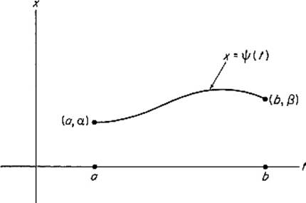
Figure 6.1

In Section 3 we will show that, if maximizes (or minimizes) the function defined by (*), subject to the conditions φ(a) = α and φ(b) = β, then φ satisfies the Euler–Lagrange equation

The proof of this will involve a generalized version of the familiar technique of “setting the derivative equal to zero, and then solving for the unknown.”

In Section 4 we discuss the so-called “isoperimetric problem,” in which it is desired to maximize or minimize the function

subject to the conditions ψ(a) = α, ψ(b) = β and the “constraint”

Here f and g are given functions on ³. We will see that, if is a solution for this problem, then there exists a number such that φ satisfies the Euler–Lagrange equation

for the function h : ³ → defined by

This assertion is reminiscent of the constrained maximum–minimum problems of Section II.5, and its proof will involve a generalization of the Lagrange multiplier method that was employed there.

As preparation for these general maximum–minimum methods, we need to develop the rudiments of “calculus in normed vector spaces.” This will be done in Sections 1 and 2.

Chapter 1. NORMED VECTOR SPACES AND UNIFORM CONVERGENCE

The introductory remarks above indicate that certain typical calculus of variations problems lead to a consideration of “function spaces” such as the vector space of all continuously differentiable functions defined on the interval [a, b]. It will be important for our purpose to define a norm on the vector space , thereby making it into a normed vector space. As we will see in Section 2, this will make it possible to study real-valued functions on by the methods of differential calculus.

Recall (from Section I.3) that a norm on the vector space V is a real-valued function x → x on V satisfying the following conditions:

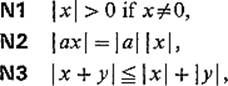
for all and . The norm x of the vector may be thought of as its length or “size.” Also, given , the norm x − y of x − y may be thought of as the “distance” from x to y.

Example 1 We have seen in Section I.3 that each of the following definitions gives a norm on ⁿ:

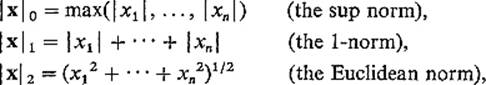
where . It was (and is) immediate that ₀ and ₁ are norms on ⁿ, while the verification that ₂ satisfies the triangle inequality (Condition N3) required the Cauchy–Schwarz inequality (Theorem I.3.1).

Any two norms on ⁿ are equivalent in the following sense. The two norms ₁ and ₂ on the vector space V are said to be equivalent if there exist positive numbers a and b such that

for all . We leave it as an easy exercise for the reader to check that this relation between norms on V is an equivalence relation (in particular, if the norms ₁ and ₂ on V are equivalent, and also ₂ and ₃ are equivalent, then it follows that ₁ and ₃ are equivalent norms on V).

We will not include here the full proof that any two norms on ⁿ are equivalent. However let us show that any continuous norm on ⁿ (that is, x is a continuous function of x) is equivalent to the Euclidean norm ₂. Since is continuous on the unit sphere

there exist positive numbers m and M such that

for all . Given , choose a > 0 such that x = ay with . Then the above inequality gives

so

as desired. In particular, the sup norm and the 1-norm of Example 1 are both equivalent to the Euclidean norm, since both are obviously continuous. For the proof that every norm on ⁿ is continuous, see Exercise 1.7.

Equivalent norms on the vector space V give rise to equivalent notions of sequential convergence in V. The sequence of points of V is said to converge to with respect to the norm if and only if

Lemma 1.1 Let ₁ and ₂ be equivalent norms on the vector space V. Then the sequence converges to with respect to the norm ₁ if and only if it converges to x with respect to the norm ₂.

This follows almost immediately from the definitions; the easy proof is left to the reader.

Example 2 Let V be the vector space of all continuous real-valued functions on the closed interval [a, b], with the vector space operations defined by

where and . We can define various norms on V, analogous to the norms on ⁿ in Example 1, by

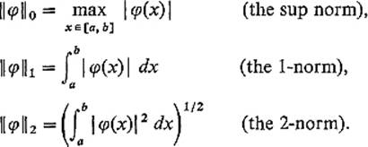
Again it is an elementary matter to show that ₀ and ₁ are indeed norms on V, while the verification that ₂ satisfies the triangle inequality requires the Cauchy–Schwarz inequality (see the remarks following the proof of Theorem 3.1 in Chapter I). We will denote by the normed vector space V with the sup norm ₀.

No two of the three norms in Example 2 are equivalent. For example, to show that ₀ and ₁ are not equivalent, consider the sequence of elements of V defined by

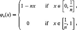
and let φ₀(x) = 0 for (here the closed interval [a, b] is the unit interval [0, 1]). Then it is clear that converges to φ₀ with respect to the 1-norm ₁ because

However does not converge to φ₀ with respect to the sup norm ₀ because

for all n. It therefore follows from Lemma 1.1 that the norms ₀ and ₁ are not equivalent.

Next we want to prove that , the vector space of Example 2 with the sup norm, is complete. The normed vector space V is called complete if every Cauchy sequence of elements of V converges to some element of V. Just as in ⁿ, the sequence is called a Cauchy sequence if, given > 0, there exists a positive integer N such that

These definitions are closely related to the following properties of sequences of functions. Let be a sequence of real-valued functions, each defined on the set S. Then is called a uniformly Cauchy sequence (of functions on S) if, given > 0, there exists N such that

for every . We say that converges uniformly to the function f: S → if, given > 0, there exists N such that

for every .

Example 3 Consider the sequence , where f_n : [0, 1] → is the function whose graph is shown in Fig. 6.2. Then lim_n→∞ f_n(x) = 0 for every . However the sequence does not converge uniformly to its pointwise limit f(x) ≡ 0, because f_n = 1 for every n (sup norm).

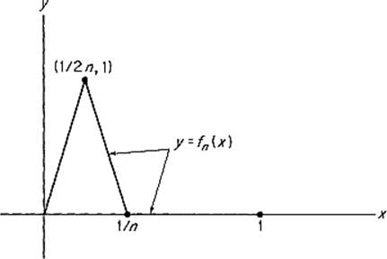
Figure 6.2

Example 4 Let f_n(x) = xⁿ on [0, 1]. Then

so the pointwise limit function is not continuous. It follows from Theorem 1.2 below that the sequence {f_n} does not converge uniformly to f.

Comparing the above definitions, note that a Cauchy sequence in is simply a uniformly Cauchy sequence of continuous functions on [a, b], and that the sequence converges with respect to the sup norm to if and only if it converges uniformly to φ. Therefore, in order to prove that is complete, we need to show that every uniformly Cauchy sequence of continuous functions on [a, b] converges uniformly to some continuous function on [a, b]. The first step is the proof that, if a sequence of continuous functions converges uniformly, then the limit function is continuous.

Theorem 1.2 Let S be a subset of ^k. Let be a sequence of continuous real-valued functions on S. If converges uniformly to the function f: S → , then f is continuous.

PROOF Given > 0, first choose N sufficiently large that f_N(x) − f(x) < /3 for all (by the uniform convergence). Then, given , choose δ > 0 such that

(by the continuity of f_N at x₀). If and x − x₀ < δ, then it follows that

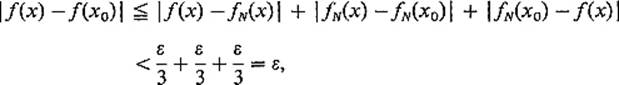
so f is continuous at x₀.

Corollary 1.3 is complete.

PROOF Let be a Cauchy sequence of elements of , that is, a uniformly Cauchy sequence of continuous real-valued functions on [a, b]. Given > 0, choose N such that

Then, in particular, φ_m(x) − φ_n(x) < /2 for each . Therefore is a Cauchy sequence of real numbers, and hence converges to some real number φ(x). It remains to show that the sequence of functions {φ_n} converges uniformly to φ; if so, Theorem 1.2 will then imply that .

We assert that (same N as above, n fixed) implies that

To see this, choose sufficiently large (depending upon x) that φ(x) − φ_m(x) < /2. Then it follows that

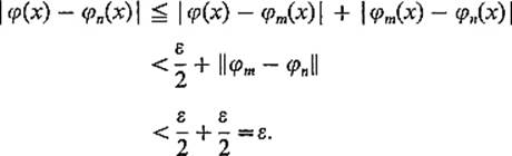
Since was arbitrary, it follows that φ_n − φ < as desired.

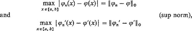
Example 5 Let denote the vector space of all continuously differentiable real-valued functions on [a, b], with the vector space operations of , but with the “-norm” defined by

for . We leave it as an exercise for the reader to verify that this does define a norm on .

In Section 4 we will need to know that the normed vector space is complete. In order to prove this, we need a result on the termwise-differentiation of a sequence of continuously differentiable functions on [a, b]. Suppose that the sequence converges (pointwise) to f, and that the sequence of derivatives converges to g. We would like to know whether f′ = g. Note that this is the question as to whether

an “interchange of limits” problem of the sort considered at the end of Section IV.3. The following theorem asserts that this interchange of limits is valid, provided that the convergence of the sequence of derivatives is uniform.

Theorem 1.4 Let be a sequence of continuously differentiable real-valued functions on [a, b], converging (pointwise) to f. Suppose that the converges uniformly to a function g. Then converges uniformly to f, and f is differentiable, with f′ = g.

PROOF By the fundamental theorem of calculus, we have

for each n and each . From this and Exercise IV.3.4 (on the termwise-integration of a uniformly convergent sequence of continuous functions) we obtain

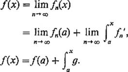
Another application of the fundamental theorem yields f′ = g as desired.

To see that the convergence of to f is uniform, note that

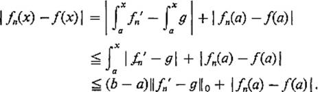
The uniform convergence of the sequence therefore follows from that of the sequence .

Corollary 1.5 is complete.

PROOF Let be a Cauchy sequence of elements of . Since

we see that is a uniformly Cauchy sequence of continuous functions. It follows from Corollary 1.3 that converges uniformly to a continuous function φ : [a, b] → . Similarly

so it follows, in the same way from Corollary 1.3, that converges uniformly to a continuous function ψ : [a, b] → . Now Theorem 1.4 implies that φ is differentiable with φ′ = ψ, so . Since

the uniform convergence of the sequences and implies that the sequence converges to φ with respect to the -norm of . Thus every Cauchy sequence in converges.

Example 6 Let denote the vector space of all paths in ⁿ (mappings φ : [a, b] → ⁿ), with the norm

where ₀ denotes the sup norm in ⁿ. Then it follows, from a coordinatewise application of Corollary 1.5, that the normed vector space is complete.

Exercises

1.1Verify that ₀, ₁, and ₂, as defined in Example 2, are indeed norms on the vector space of all continuous functions defined on [a, b].

1.2Show that the norms ₁ and ₂ of Example 2 are not equivalent. Hint: Truncate the function near 0.

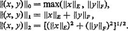
1.3Let E and F be normed vector spaces with norms _E and _F, respectively. Then the the product set E × F is a vector space, with the vector space operations defined coordinatewise. Prove that the following are equivalent norms on E × F:

1.4If the normed vector spaces E and F are complete, prove that the normed vector space E × F, of the previous exercise, is also complete.

1.5Show that a closed subspace of a complete normed vector space is complete.

1.6Denote by _n[a, b] the subspace of that consists of all polynomials of degree at most n. Show that _n[a, b] is a closed subspace of . Hint: Associate the polynomial with the point , and compare φ₀ with a.

1.7If is a norm on ⁿ, prove that the function x → x is continuous on ⁿ. Hint: If

then

The Cauchy-Schwarz inequality then gives

where and is the Euclidean norm on ⁿ.