Advanced Calculus of Several Variables (1973)
Part I. Euclidean Space and Linear Mappings
Chapter 4. LINEAR MAPPINGS AND MATRICES
In this section we introduce an important special class of mappings of Euclidean spaces—those which are linear (see definition below). One of the central ideas of multivariable calculus is that of approximating nonlinear mappings by linear ones.
Given a mapping f : ![]() n →
n → ![]() m, let f1, . . . , fm be the component functions of f. That is, f1, . . . , fm are the real-valued functions on
m, let f1, . . . , fm be the component functions of f. That is, f1, . . . , fm are the real-valued functions on ![]() n defined by writing
n defined by writing ![]() In Chapter II we will see that, if the component functions of f are continuously differentiable at
In Chapter II we will see that, if the component functions of f are continuously differentiable at ![]() , then there exists a linear mapping L :
, then there exists a linear mapping L : ![]() n →
n → ![]() m such that
m such that
![]()
with limh→0 R(h)/![]() h
h![]() = 0. This fact will be the basis of much of our study of the differential calculus of functions of several variables.
= 0. This fact will be the basis of much of our study of the differential calculus of functions of several variables.
Given vector spaces V and W, the mapping L : V → W is called linear if and and only if
![]()
for all ![]() and
and ![]() . It is easily seen (Exercise 4.1) that the mapping L satisfies (1) if and only if
. It is easily seen (Exercise 4.1) that the mapping L satisfies (1) if and only if
![]()
and
![]()
for all ![]() and
and ![]() .
.
Example 1Given ![]() , the mapping f :
, the mapping f : ![]() →
→ ![]() defined by f(x) = bx obviously satisfies conditions (2) and (3), and is therefore linear. Conversely, if f is linear, then f(x) = f(x · 1) = xf(1), so f is of the form f(x) = bx with b = f(1).
defined by f(x) = bx obviously satisfies conditions (2) and (3), and is therefore linear. Conversely, if f is linear, then f(x) = f(x · 1) = xf(1), so f is of the form f(x) = bx with b = f(1).
Example 2The identity mapping I : V → V, defined by I(x) = x for all ![]() , is linear, as is the zero mapping x → 0. However the constant mapping x → c is not linear if c ≠ 0 (why?).
, is linear, as is the zero mapping x → 0. However the constant mapping x → c is not linear if c ≠ 0 (why?).
Example 3Let f : ![]() 3 →
3 → ![]() 2 be the vertical projection mapping defined by f(x, y, z) = (x, y). Then f is linear.
2 be the vertical projection mapping defined by f(x, y, z) = (x, y). Then f is linear.
Example 4Let ![]() denote the vector space of all infinitely differentiable functions from
denote the vector space of all infinitely differentiable functions from ![]() to
to ![]() . If D(f ) denotes the derivative of
. If D(f ) denotes the derivative of ![]() then D :
then D : ![]() →
→ ![]() is linear.
is linear.
Example 5Let ![]() denote the vector space of all continuous functions on [a, b]. If
denote the vector space of all continuous functions on [a, b]. If ![]() , then
, then ![]() is linear.
is linear.
Example 6Given ![]() the mapping f :
the mapping f : ![]() 3 →
3 → ![]() defined by f(x) = a · x = a1 x1 + a2 x2 + a3 x3 is linear, because a · (x + y) = a · x + a · y and a · (cx) = c(a · x).
defined by f(x) = a · x = a1 x1 + a2 x2 + a3 x3 is linear, because a · (x + y) = a · x + a · y and a · (cx) = c(a · x).
Conversely, the approach of Example 1 can be used to show that a function f: ![]() 3 →
3 → ![]() is linear only if it is of the form f(x1, x2, x3) = a1 x1 + a2 x2 + a3 x3. In general, we will prove in Theorem 4.1 that the mapping f:
is linear only if it is of the form f(x1, x2, x3) = a1 x1 + a2 x2 + a3 x3. In general, we will prove in Theorem 4.1 that the mapping f: ![]() n →
n → ![]() m is linear if and only if there exist numbers aij, i = 1, . . . , m, j = 1, . . . , n, such that the coordinate functions f1, . . . , fm of f are given by
m is linear if and only if there exist numbers aij, i = 1, . . . , m, j = 1, . . . , n, such that the coordinate functions f1, . . . , fm of f are given by
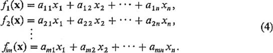
for all ![]() . Thus the linear mapping f is completely determined by the rectangular array
. Thus the linear mapping f is completely determined by the rectangular array
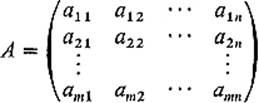
of numbers. Such a rectangular array of real numbers is called a matrix. The horizontal lines of numbers in a matrix are called rows; the vertical ones are called columns. A matrix having m rows and n columns is called an m × nmatrix. Rows are numbered from top to bottom, and columns from left to right. Thus the element aij of the matrix A above is the one which is in the ith row and the jth column of A. This type of notation for the elements of a matrix is standard—the first subscript gives the row and the second the column. We frequently write A = (aij) for brevity.
The set of all m × n matrices can be made into a vector space as follows. Given two m × n matrices A = (aij) and B = (bij), and a number r, we define
![]()
That is, the ijth element of A + B is the sum of the ijth elements of A and B, and the ijth element of rA is r times that of A. It is a simple matter to check that these two definitions satisfy conditions V1–V8 of Section 1.
Indeed these operations for matrices are simply an extension of those for vectors. A 1 × n matrix is often called a row vector, and an m × 1 matrix is similarly called a column vector. For example, the ith row
![]()
of the matrix A is a row vector, and the jth column
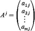
of A is a column vector. In terms of the rows and columns of a matrix A, we will sometimes write

using subscripts for rows and superscripts for columns.
Next we define an operation of multiplication of matrices which generalizes the inner product for vectors. We define the product AB first in the special case when A is a row vector and B is a column vector of the same dimension. If
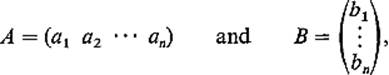
we define ![]() Thus in this case AB is just the scalar product of A and B as vectors, and is therefore a real number (which we may regard as a 1 × 1 matrix).
Thus in this case AB is just the scalar product of A and B as vectors, and is therefore a real number (which we may regard as a 1 × 1 matrix).
The product AB in general is defined only when the number of columns of A is equal to the number of rows of B. So let A = (aij) be an m × n matrix, and B = (bij) an n × p matrix. Then the product AB of A and B is by definition the m × p matrix
![]()
whose ijth element is the product of the ith row of A and the jth column of B (note that it is the fact that the number of columns of A equals the number of rows of B which allows the row vector Ai and the column vector Bj to be multiplied). The product matrix AB then has the same number of rows as A, and the same number of columns as B. If we write AB = (cij), then this product is given in terms of matrix elements by
![]()
So as to familiarize himself with the definition completely, the student should multiply together several suitable pairs of matrices.
Let us note now that Eqs. (4) can be written very simply in matrix notation. In terms of the ith row vector Ai of A and the column vector
the ith equation of (4) becomes
![]()
Consequently, by the definition of matrix multiplication, the m scalar equations (4) are equivalent to the single matrix equation
![]()
so that our linear mapping from ![]() n to
n to ![]() m takes a form which in notation is precisely the same as that for a linear real-valued function of one variable [f(x) = ax]. Of course f(x) on the left-hand side of (7) is a column vector, like xon the right-hand side. In order to take advantage of matrix notation, we shall hereafter regard points of
m takes a form which in notation is precisely the same as that for a linear real-valued function of one variable [f(x) = ax]. Of course f(x) on the left-hand side of (7) is a column vector, like xon the right-hand side. In order to take advantage of matrix notation, we shall hereafter regard points of ![]() n interchangeably as n-tuples or n-dimensional column vectors; in all matrix contexts they will be the latter. The fact that (Eqs. (4) take the simple form (7) in terms of matrices, together with the fact that multiplication as defined by (5) turns out to be associative (Theorem 4.3 below), is the main motivation for the definition of matrix multiplication.
n interchangeably as n-tuples or n-dimensional column vectors; in all matrix contexts they will be the latter. The fact that (Eqs. (4) take the simple form (7) in terms of matrices, together with the fact that multiplication as defined by (5) turns out to be associative (Theorem 4.3 below), is the main motivation for the definition of matrix multiplication.
Now let an m × n matrix A be given, and define a function f: ![]() n →
n → ![]() m by f(x) = Ax. Then f is linear, because
m by f(x) = Ax. Then f is linear, because
![]()
by the distributivity of the scalar product of vectors, so f(x + y) = f(x) + f(y), and f(rx) = rf(x) similarly. The following theorem asserts not only that every mapping of the form f(x) = Ax is linear, but conversely that every linear mapping from ![]() n to
n to ![]() m is of this form.
m is of this form.
Theorem 4.1The mapping f: ![]() n →
n → ![]() m is linear if and only if there exists a matrix A such that f(x) = Ax for all
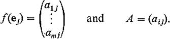
m is linear if and only if there exists a matrix A such that f(x) = Ax for all ![]() . Then A is that m × n matrix whose jth column is the column vector f(ej), where ej = (0, . . . , 1, . . . , 0) is the jth unit vector in
. Then A is that m × n matrix whose jth column is the column vector f(ej), where ej = (0, . . . , 1, . . . , 0) is the jth unit vector in ![]() n.
n.
PROOFGiven the linear mapping f: ![]() n →
n → ![]() m, write
m, write
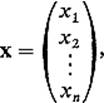
Then, given x = (x1, . . . , xn) = x1 e1 + · · · + xn en in ![]() n, we have
n, we have
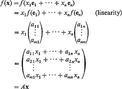
as desired.
![]()
Example 7If f: ![]() n →
n → ![]() 1 is a linear function on
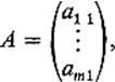
1 is a linear function on ![]() n, then the matrix A provided by the theorem has the form
n, then the matrix A provided by the theorem has the form
![]()
Hence, deleting the first subscript, we have
![]()
Thus the linear mapping f: ![]() n →
n → ![]() 1 can be written
1 can be written
![]()
where ![]()
Example 8If f: ![]() 1 →
1 → ![]() m is a linear mapping, then the matrix A has the form
m is a linear mapping, then the matrix A has the form
Writing ![]() (second subscripts deleted), we then have
(second subscripts deleted), we then have
![]()
for all ![]() . The image under f of
. The image under f of ![]() 1 in
1 in ![]() m is thus the line through 0 in
m is thus the line through 0 in ![]() m determined by a.
m determined by a.
Example 9The matrix which Theorem 4.1 associates with the identity transformation
![]()
of ![]() n is the n × n matrix
n is the n × n matrix
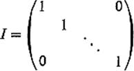
having every element on the principal diagonal (all the elements aij with i = j) equal to 1, and every other element zero. I is called the n × n identity matrix. Note that AI = IA = A for every n × n matrix A.
Example 10Let R(α): ![]() 2 →
2 → ![]() 2 be a counterclockwise rotation of
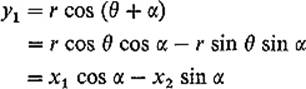
2 be a counterclockwise rotation of ![]() 2 about 0 through the angle α (Fig. 1.4). We show that R(α) is linear by computing its matrix explicitly. If (r, θ) are the polar coordinates of x = (x1, x2), so
2 about 0 through the angle α (Fig. 1.4). We show that R(α) is linear by computing its matrix explicitly. If (r, θ) are the polar coordinates of x = (x1, x2), so
![]()
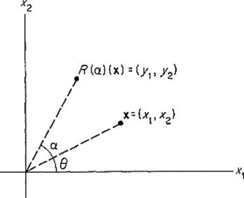
Figure 1.4
then the polar coordinates of (y1, y2) = R(α)(x) are (r, θ + α), so
and
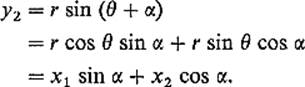
Therefore
![]()
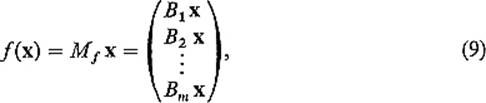
Theorem 4.1 sets up a one-to-one correspondence between the set of all linear maps f: ![]() n →
n → ![]() m and the set of all m × n matrices. Let us denote by Mf the matrix of the linear map f.
m and the set of all m × n matrices. Let us denote by Mf the matrix of the linear map f.
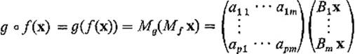
The following theorem asserts that the problem of finding the composition of two linear mappings is a purely computational matter—we need only multiply their matrices.
Theorem 4.2If the mappings f : ![]() n →
n → ![]() m and g :
m and g : ![]() m →
m → ![]() p are linear, then so is g
p are linear, then so is g ![]() f :
f : ![]() n →
n → ![]() p, and
p, and
![]()
PROOFLet Mg = (aij) and Mf = (bij). Then Mg Mf = (Ai Bj), where Ai is the ith row of Mg and Bj is the jth column of Mf. What we want to prove is that
![]()
that is, that
![]()
where x = (x1, . . . , xn) and g ![]() f(x) = (z1, . . . , zp). Now
f(x) = (z1, . . . , zp). Now
where Bk = (bk1 · · · bkn) is the kth row of Mf, so
![]()
Also
using (9). Therefore
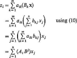
as desired [recall (8)]. In particular, since we have shown that g ![]() f(x) = (Mg Mf)x, it follows from Theorem 4.1 that g
f(x) = (Mg Mf)x, it follows from Theorem 4.1 that g ![]() f is linear.
f is linear.
![]()
Finally, we list the standard algebraic properties of matrix addition and multiplication.
Theorem 4.3Addition and multiplication of matrices obey the following rules:
(a)A(BC) = (AB)C (associativity).
(b)A(B + C) = AB + AC
(c)(A + B)C = AC + BC} (distributivity).
(d)(rA)B = r(AB) = A(rB).
PROOFWe prove (a) and (b), leaving (c) and (d) as exercises for the reader.
Let the matrices A, B, C be of dimensions k × l, l × m, and m × n respectively. Then let f : ![]() 1 →
1 → ![]() k, g :
k, g : ![]() m →
m → ![]() l, h :
l, h : ![]() n →
n → ![]() m be the linear maps such that Mf = A, Mg = B, Mh = C. Then
m be the linear maps such that Mf = A, Mg = B, Mh = C. Then
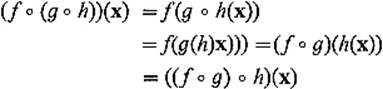
for all ![]() , so f
, so f ![]() (g
(g ![]() h) = (f
h) = (f ![]() g)
g) ![]() h. Theorem 4.2 therefore implies that
h. Theorem 4.2 therefore implies that
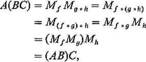
thereby verifying associativity.
To prove (b), let A be an l × m matrix, and B, C m × n matrices. Then let f : ![]() m →
m → ![]() l and g, h :
l and g, h : ![]() n →
n → ![]() m be the linear maps such that Mf = A, Mg = B, and Mh = C. Then f
m be the linear maps such that Mf = A, Mg = B, and Mh = C. Then f ![]() (g + h) = f
(g + h) = f ![]() g + f
g + f ![]() h, so Theorem 4.2 and Exercise 4.9give
h, so Theorem 4.2 and Exercise 4.9give
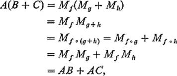
thereby verifying distributivity.
![]()
The student should not leap from Theorem 4.3 to the conclusion that the algebra of matrices enjoys all of the familiar properties of the algebra of real numbers. For example, there exist n × n matrices A and B such that AB ≠ BA, so the multiplication of matrices is, in general, not commutative (see Exercise 4.12). Also there exist matrices A and B such that AB = 0 but neither A nor B is the zero matrix whose elements are all 0 (see Exercise 4.13). Finally not every non-zero matrix has an inverse (see Exercise 4.14). The n × n matrices A and B are called inverses of each other if AB = BA = I.
Exercises
4.1Show that the mapping f : V → W is linear if and only if it satisfies conditions (2) and (3).
4.2Tell whether or not f : ![]() 3 →
3 → ![]() 2 is linear, if f is defined by
2 is linear, if f is defined by
(a)f(x, y, z) = (z, x),
(b)f(x, y, z) = (xy, yz),
(c)f(x, y, z) = (x + y, y + z),
(d)f(x, y, z) = (x + y, z + 1),
(e)f(x, y, z) = (2x − y − z, x + 3y + z).
For each of these mappings that is linear, write down its matrix.
4.3Show that, if b ≠ 0, then the function f(x) = ax + b is not linear. Although such functions are sometimes loosely referred to as linear ones, they should be called affine—an affine function is the sum of a linear function and a constant function.
4.4Show directly from the definition of linearity that the composition g ![]() f is linear if both f and g are linear.
f is linear if both f and g are linear.
4.5Prove that the mapping f : ![]() n →
n → ![]() m is linear if and only if its coordinate functions f1, . . . . , fm are all linear.
m is linear if and only if its coordinate functions f1, . . . . , fm are all linear.
4.6The linear mapping L : ![]() n →
n → ![]() n is called norm preserving if
n is called norm preserving if ![]() L(x)
L(x)![]() =
= ![]() x
x![]() , and inner product preserving if L(x) • L(y) = x • y. Use Exercise 3.5 to show that L is norm preserving if and only if it is inner product preserving.
, and inner product preserving if L(x) • L(y) = x • y. Use Exercise 3.5 to show that L is norm preserving if and only if it is inner product preserving.
4.7Let R(α) be the counterclockwise rotation of ![]() 2 through an angle α. Then, as shown in Example 10, the matrix of R(α) is
2 through an angle α. Then, as shown in Example 10, the matrix of R(α) is
![]()
It is geometrically clear that R(α) ![]() R(β) = R(α + β), so Theorem 4.2 gives MR(α) MR(β) = MR(α + β). Verify this by matrix multiplication.
R(β) = R(α + β), so Theorem 4.2 gives MR(α) MR(β) = MR(α + β). Verify this by matrix multiplication.
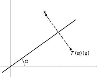
Figure 1.5
4.8Let T(α): ![]() 2 →
2 → ![]() 2 be the reflection in
2 be the reflection in ![]() 2 through the line through 0 at an angle α from the horizontal (Fig. 1.5). Note that T(0) is simply reflection in the x1-axis, so
2 through the line through 0 at an angle α from the horizontal (Fig. 1.5). Note that T(0) is simply reflection in the x1-axis, so
![]()
Using the geometrically obvious fact that T(α) = R(α) ![]() T(0)
T(0) ![]() R(−α), apply Theorem 4.2 to compute MT(α) by matrix multiplication.
R(−α), apply Theorem 4.2 to compute MT(α) by matrix multiplication.
4.9Show that the composition of two reflections in ![]() 2 is a rotation by computing the matrix product MT(α)MT(β). In particular, show that MT(α)MT(β) = MR(γ) for some γ, identifying γ in terms of α and β.
2 is a rotation by computing the matrix product MT(α)MT(β). In particular, show that MT(α)MT(β) = MR(γ) for some γ, identifying γ in terms of α and β.
4.10If f and g are linear mappings from ![]() n to
n to ![]() m, show that f + g is also linear, with Mf + g = Mf + Mg.
m, show that f + g is also linear, with Mf + g = Mf + Mg.
4.11Show that (A + B)C = AC + BC by a proof similar to that of part (b) of Theorem 4.3.
4.12If f = R(π/2), the rotation of ![]() 2 through the angle π/2, and g = T(0), reflection of
2 through the angle π/2, and g = T(0), reflection of ![]() 2 through the x1-axis, then g(f(1, 0)) = (0, −1)), while f(g(1, 0)) = (0, 1). Hence it follows from Theorem 4.2 that MgMf ≠ MfMg. Consulting Exercises 4.7 and 4.8 for Mf and Mg, verify this by matrix multiplication.
2 through the x1-axis, then g(f(1, 0)) = (0, −1)), while f(g(1, 0)) = (0, 1). Hence it follows from Theorem 4.2 that MgMf ≠ MfMg. Consulting Exercises 4.7 and 4.8 for Mf and Mg, verify this by matrix multiplication.
4.13Find two linear maps f, g: ![]() 2 →
2 → ![]() 2, neither identically zero, such that the image of f and the kernel of g are both the x1-axis. Then Mf and Mg will be nonzero matrices such that MgMf = 0. Verify this by matrix multiplication.
2, neither identically zero, such that the image of f and the kernel of g are both the x1-axis. Then Mf and Mg will be nonzero matrices such that MgMf = 0. Verify this by matrix multiplication.
4.14Show that, if ad = bc, then the matrix ![]() has no inverse.
has no inverse.
4.15If ![]() and
and ![]() , compute AB and BA. Conclude that, if ad − bc ≠ 0, then A has an inverse.
, compute AB and BA. Conclude that, if ad − bc ≠ 0, then A has an inverse.
4.16Let P(α), Q(α), and R(α) denote the rotations of ![]() 3 through an angle α about the x1-, x2-, and x3-axes respectively. Using the facts that
3 through an angle α about the x1-, x2-, and x3-axes respectively. Using the facts that
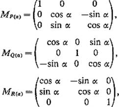
show by matrix multiplication that
![]()