Advanced Calculus of Several Variables (1973)

Part I. Euclidean Space and Linear Mappings

Chapter 7. LIMITS AND CONTINUITY

We now generalize to higher dimensions the familiar single-variable definitions of limits and continuity. This is largely a matter of straightforward repetition, involving merely the use of the norm of a vector in place of the absolute value of a number.

Let D be a subset of ⁿ, and f a mapping of D into ^m (that is, a rule that associates with each point a point . We write f: D → ^m, and call D the domain (of definition) of f.

In order to define lim_x→a f(x), the limit of f at a, it will be necessary that f be defined at points arbitrarily close to a, that is, that D contains points arbitrarily close to a. However we do not want to insist that , that is, that f be defined at a. For example, when we define the derivative f′(a) of a real-valued single-variable function as the limit of its difference quotient at a,

this difference quotient is not defined at a.

This consideration motivates the following definition. The point a is a limit point of the set D if and only if every open ball centered at a contains points of D other than a (this is what is meant by the statement that D contains points arbitrarily close to a). By the open ball of radius r centered at a is meant the set

Note that a may, or may not, be itself a point of D. Examples: (a) A finite set of points has no limit points; (b) every point of ⁿ is a limit point of ⁿ (c) the origin 0 is a limit point of the set ⁿ − 0; (d) every point of ⁿ is a limit point of the set Q of all those points of ⁿ having rational coordinates; (e) the closed ball

is the set of all limit points of the open ball B_r(a).

Given a mapping f: D → ^m, a limit point a of D, and a point , we say that b is the limit of f at a, written

if and only if, given > 0, there exists δ > 0 such that and 0 < x − a < δ imply f(x) − b < .

The idea is of course that f(x) can be made arbitrarily close to b by choosing x sufficiently close to a, but not equal to a. In geometrical language (Fig. 1.6),

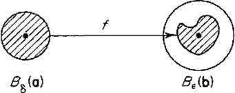
Figure 1.6

the condition of the definition is that, given any open ball B(b) centered at b, there exists an open ball B_δ(a) centered at a, whose intersection with D − a is sent by f into B(b).

Example 1Consider the function f: ² → defined by

In order to prove that lim_x→(1,1) f(x, y) = 3, we first write

Given > 0, we want to find δ > 0 such that (x, y) − (1, 1) = [(x − 1)² + (y − 1)²]^1/2 < δ implies that the right-hand side of (1) is < . Clearly we need bounds for the coefficients x + 1 and y of x − 1 in (1). So let us first agree to choose , so

which then implies that

by (1). It is now clear that, if we take

then

as desired.

Example 2Consider the function f: ² → defined by

To investigate lim_(x,y)→0 f(x, y), let us consider the value of f(x, y) as (x, y) approaches 0 along the straight line y = αx. The lines y = ±x, along which f(x, y) = 0, are given by α = ±1. If α ≠ ±1, then

For instance,

for all x ≠ 0. Thus f(x, y) has different constant values on different straight lines through 0, so it is clear that lim_(x,y)→0 f(x, y) does not exist (because, given any proposed limit b, the values and of f cannot both be within of b if ).

Example 3Consider the function f: → ² defined by f(t) = (cos t, sin t), the familiar parametrization of the unit circle. We want to prove that

Given > 0, we must find δ > 0 such that

In order to simplify the square root, write a = cos t − 1 and b = sin t. Then

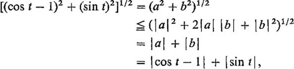
so we see that it suffices to find δ > 0 such that

But we can do this by the fact (from introductory calculus) that the functions cos t and sin t are continuous at 0 (where cos 0 = 1, sin 0 = 0).

Example 3 illustrates the fact that limits can be evaluated coordinatewise. To state this result precisely, consider f: D → ^m, and write for each . Then f₁, . . . , f_m are real-valued functions on D, called as usual the coordinate functions of f, and we write f = (f₁, . . . , f_m). For the function f of Example 3 we have f = (f₁, f₂) where f₁(t) = cos t, f₂(t) = sin t, and we found that

Theorem 7.1Suppose f = (f₁, . . . , f_m): D → _m, that a is a limit point of D, and . Then

if and only if

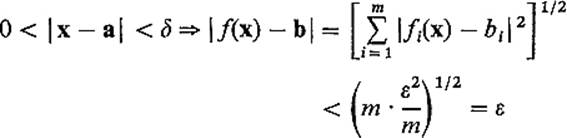
PROOFFirst assume (2). Then, given > 0, there exists δ > 0 such that and 0 < x − a < δ imply that f(x) − b < . But then

so (3) holds for each i = 1, . . . , m.

Conversely, assume (3). Then, given > 0, for each i = 1, . . . , m there exists a δ_i > 0 such that

If we now choose δ = min(δ₁, . . . , δ_m), then and

by (4), so we have shown that (3) implies (2).

The student should recall the concept of continuity introduced in single-variable calculus. Roughly speaking, a continuous function is one which has nearby values at nearby points, and thus does not change values abruptly. Precisely, the function f: D → ^m is said to be continuous at if and only if

f is said to be continuous on D (or, simply, continuous) if it is continuous at every point of D.

Actually we cannot insist upon condition (5) if is not a limit point of D, for in this case the limit of f at a cannot be discussed. Such a point, which belongs to D but is not a limit point of D, is called an isolated point of D, and we remedy this situation by including in the definition the stipulation that f is automatically continuous at every isolated point of D.

Example 4If D is the open ball B₁(0) together with the point (2, 0), then any function f on D is continuous at (2, 0), while f is continuous at if and only if condition (5) is satisfied.

Example 5If D is the set of all those points (x, y) of ² such that both x and y are integers, then every point of D is an isolated point, so every function on D is continuous (at every point of D).

The following result is an immediate corollary to Theorem 7.1.

Theorem 7.2The mapping f: D → ^m is continuous at if and only if each coordinate function of f is continuous at a.

Example 6The identity mapping π : ⁿ → ⁿ, defined by π(x) = x, is obviously continuous. Its ith coordinate function, π_i(x₁, . . . , x_n) = x_i, is called the ith projection function, and is continuous by Theorem 7.2.

Example 7The real-valued functions s and p on ², defined by s(x, y) = x + y and p(x, y) = xy, are continuous. The proofs are left as exercises.

The continuity of many mappings can be established without direct recourse to the definition of continuity—instead we apply the known continuity of the elementary single-variable functions, elementary facts such as Theorem 7.2 and Examples 6 and 7, and the fact that a composition of continuous functions is continuous. Given f : D₁ → ^m and g : D₂ → ^k, where and , the composition

of f and g is defined as usual by g f(x) = g(f(x)) for all such that and . That is, the domain of g f is

(This is simply the set of all x such that g(f(x)) is meaningful.)

Theorem 7.3If f is continuous at a and g is continuous at f(a), then g f is continuous at a.

This follows immediately from the following lemma [upon setting b = f(a)].

Lemma 7.4Given f : D₁ → ^m and g: D₂ → ^k where and , suppose that

and that

Then

PROOFGiven > 0, we must find δ > 0 such that g(f(x)) − g(b) < if 0 < x − a < δ and , the domain of g f. By (7) there exists η > 0 such that

Then by (6) there exists δ > 0 such that

But then, upon substituting y = f(x) in (8), we obtain

as desired.

It may be instructive for the student to consider also the following geometric formulation of the proof of (Theorem 7.3 see Fig. 1.7).

Given > 0, we want δ > 0 so that

Since g is continuous at f(a), there exists η > 0 such that

Then, since f is continuous at a, there exists δ > 0 such that

Then

as desired.

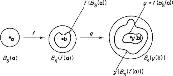
Figure 1.7

As an application of the above results, we now prove the usual theorem on limits of sums and products without mentioning and δ.

Theorem 7.5Let f and g be real-valued functions on ⁿ. Then

and

provided that lim_{x → a} f(x) and lim_x→a g(x) exist.

PROOFWe prove (9), and leave the similar proof of (10) to the exercises. Note first that

where s(x, y) = x + y is the sum function on ² of Example 7. If

then lim_x→a (f(x), g(x)) = (b₁, b₂) by Theorem 7.1, so

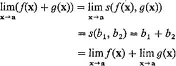
by Lemma 7.4.

Example 8It follows by mathematical induction from Theorem 7.5 that a sum of products of continuous functions is continuous. For instance, any linear real-valued function

or polynomial in x₁, . . . , x_n, is continuous. It then follows from Theorem 7.1 that any linear mapping L : ⁿ → ^m is continuous.

Example 9To see that f : ³ → , defined by f(x, y, z) = sin(x + cos yz), is continuous, note that

where π₁, π₂, π₃ are the projection functions on ³, and s and p are the sum and product functions on ².

Exercises

7.1Verify that the functions s and p of Example 7 are continuous. Hint: xy − x₀y₀ = (xy − xy₀) + (xy₀ − x₀y₀).

7.2Give an − δ proof that the function f: ³ → defined by f(x, y, z) = x²y + 2xz² is continuous at (1, 1, 1). Hint: x²y + 2xz² − 3 = (x²y − y) + (y − 1) + (2xz² − 2x) + (2x − 2).

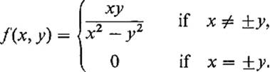
7.3If f(x, y) = (x² − y²)/(x² + y²) unless x = y = 0, and f(0, 0) = 0, show that f: ² → is not continuous at (0, 0). Hint: Consider the behavior of f on straight lines through the origin.

7.4Let f(x, y) = 2x²y/(x⁴ + y²) unless x = y = 0, and f(0, 0) = 0. Define φ(t) = (t, at) and ψ(t) = (t, t²).

(a)Show that lim_t→0 f(φ(t)) = 0. Thus f is continuous on any straight line through (0, 0).

(b)Show that lim_t→0 f(ψ(t)) = 1. Conclude that f is not continuous at (0, 0).

7.5Prove the second part of Theorem 7.5.

7.6The point a is called a boundary point of the set if and only if every open ball centered at a contains both a point of D and a point of the complementary set ⁿ − D.

For example, the set of all boundary points of the open ball B_r(p) is the sphere . Show that every boundary point of D is either a point of D or a limit point of D.

7.7Let D^* denote the set of all limit points of the set D^*. Then prove that the set contains all of its limit points.

7.8Let f: ⁿ → ^m be continuous at the point a. If is a sequence of points of ⁿ which converges to a, prove that the sequence converges to the point f(a).