High School Algebra II Unlocked (2016)
Chapter 3. Radical and Rational Equations and Inequalities
Lesson 3.3. Rational Functions
REVIEW
The domain of a function is the set of x-values, or input values, for which the function exists.
An even function is a function f(x) for which f(−x) = f(x). The graph of an even function is symmetrical with respect to the y-axis.
An inverse variation is a variation equation in which one variable is inversely proportional to the other variable. If a is inversely proportional to b, then a = k/b, where k is some constant.
An odd function is a function f(x) for which f(−x) = −f(x). The graph of an odd function is symmetrical with respect to the origin.
The range of a function is the set of output values (generally y-values or f(x)-values) corresponding to the x-values in the domain of the function. The x- and y-intercepts are points of intersection within the x- and y-axis (respectively).
A rational function is a function that is defined as a rational expression, a ratio of one polynomial to another.
One very simple type of rational function is an inverse variation relationship.

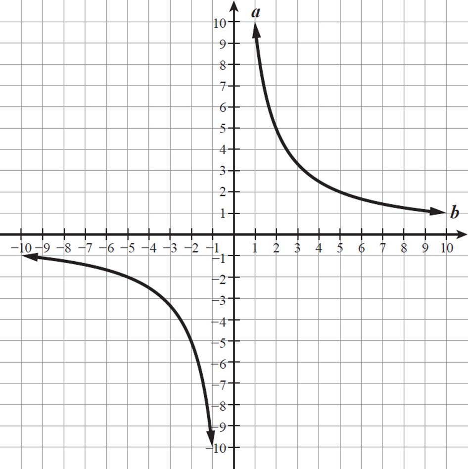
In the function a = 10/b, what happens to a as b approaches positive and negative infinity? Graph this function.
As the value of b increases, 10/b becomes a smaller and smaller positive fraction. As b approaches infinity (∞), a approaches 0.
If b were a negative number decreasing to negative infinity (−∞), then a would be a negative number, but it would still be getting closer and closer to 0. (For example, when b = −1000, a = −1/100.)
Use the equation to find more coordinate pairs on the graph.
|
When b = 1, a = 10. |
When b = −1, a = −10. |
|
When b = 5, a = 2. |
When b = −5, a = −2. |
|
When b = 10, a = 1. |
When b = −10, a = −1. |
So, the graph of a = 10/b passes through (1, 10), (5, 2), (10, 1), (−1, −10), (−5, −2), and (−10, −1).
Let’s also look at what happens when the value of b is close to 0. When b = 0, the fraction 10/b is undefined, so a does not exist when b = 0. As b approaches 0 as a positive number, the value of 10/b becomes very large. As b approaches 0 as a negative number, the value of 10/b is negative but with a large absolute value. So, as b approaches 0 from the right on the graph, a approaches infinity, and as b approaches 0 from the left, a approaches negative infinity.
The graph of a = 10/b is shown below.
Notice that this graph
is symmetrical with
respect to the origin.
This is because the
function a = 10/b is
an odd function. If
you substitute −b for
b, the result is −a.

There is a vertical asymptote at b = 0, or the a-axis. The function a = 10/b approaches −∞ on the left side and ∞ on the right side as b nears 0. The function will never intersect the a-axis. It just continually gets closer and closer to it.
There is a horizontal asymptote at a = 0, or the b-axis. Both ends of the function a = 10/b approach this line, as b approaches −∞ and ∞. The function value gets closer and closer to 0 but never reaches it.
Even if the equation in Example 7 had a more complicated denominator, such as a = 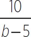 , both ends of the function a would still approach a horizontal asymptote of a = 0 as b approaches positive and negative infinity. A difference of 5 is basically meaningless when b has a huge absolute value.
Let’s look at some more complicated rational functions.

Here is how you may see rational functions on the ACT.
In the equation a = 5/b, b is a positive real number. As the value of b is increased so it becomes closer and closer to infinity, what happens to the value of a?
A. It remains constant.
B. It gets closer and closer to zero.
C. It gets closer and closer to one.
D. It gets closer and closer to five.
E. It gets closer and closer to infinity.

Create tables of values and graph each of the functions below.
|
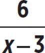
f(x) = |
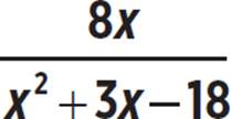
g(x) = |
For each rational function, we’ll need more points to get a sense of the graph’s behavior than we would for a linear or quadratic function.
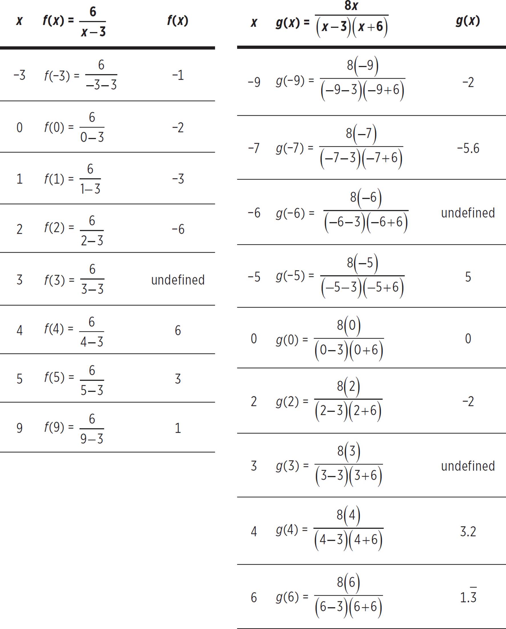
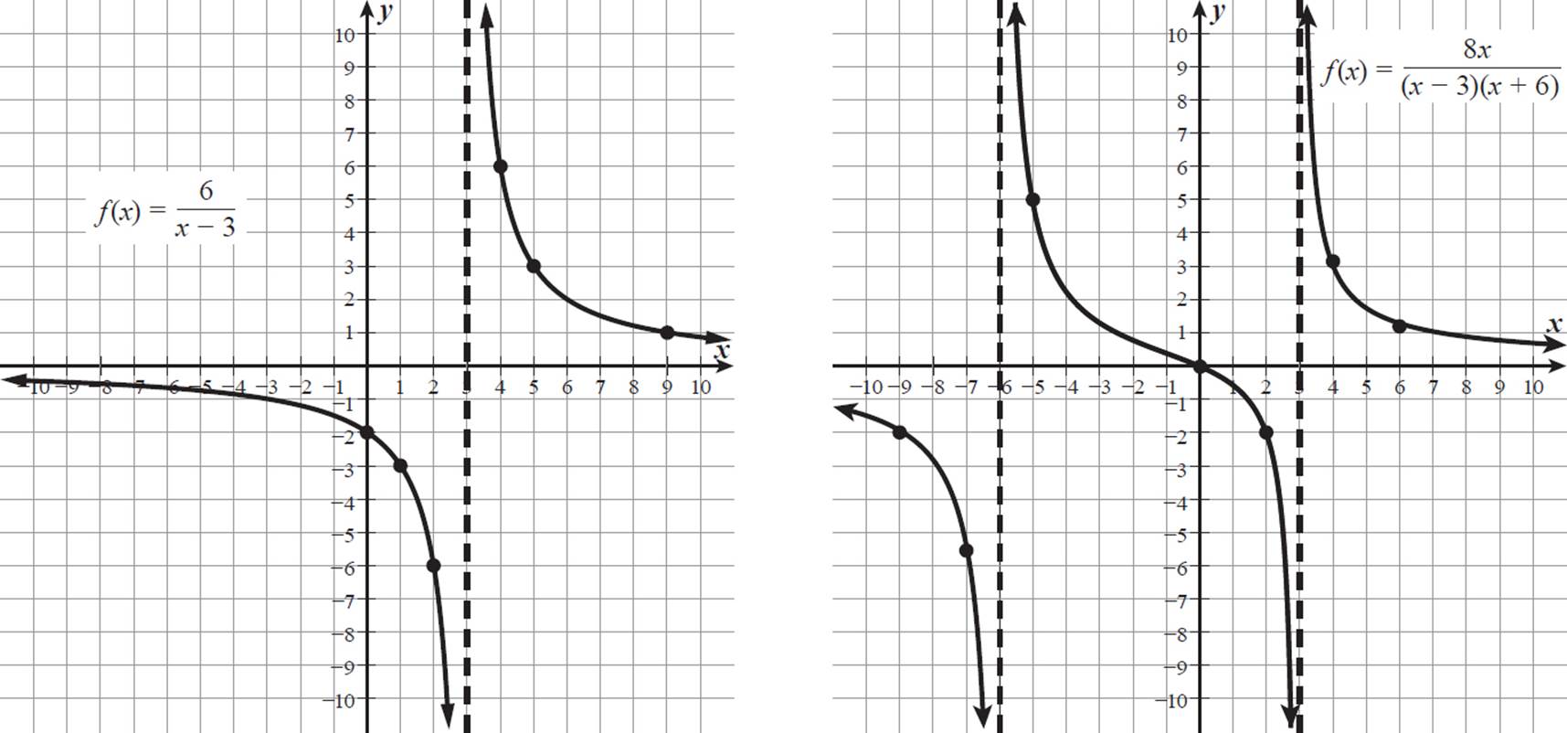
It’s clear from these tables that something funny happens to each function around the point(s) where it is undefined. The graph drops as it approaches one of those points from the left (increasing x-values), but on the right side it is suddenly much higher and dropping again. These places involve vertical asymptotes, such as the one in Example 7. Let’s look at the complete graph of each of these functions, as shown on a graphing calculator, passing through the points we found.
Although these
particular functions are
constantly decreasing
over each continuous
section, some rational
functions increase over
some or all of their
continuous sections.


To see what happens, we can plug in increasing positive values of b and solve for a.
When b = 1, a = 5.
When b = 5, a = 1.
When b = 50, a = 1/10.
When b = 500, a = 1/100.
When b = 5000, a = 1/1000.
Even though a reaches values of 5 and 1, which are listed in the answer choices, the question asks only for what happens to a as b approaches infinity.
As the value of b increases, the value of a decreases. It never becomes negative, though. It just becomes a smaller and smaller fraction. In other words, as b approaches infinity (∞), a approaches 0. The correct answer is (B).
The dashed lines indicate where there are vertical asymptotes. The graph approaches these lines but never actually intersects them. These are points of discontinuity for the graphs. Notice that they are exactly at the x-values where f(x) and g(x) are undefined. As with the function in Example 7, when the denominator approaches 0, the function value nears either positive or negative infinity.
The graph of f(x) =  has an unmarked horizontal asymptote at the x-axis, or where f(x) = 0. Although it approaches 0, f(x) never actually reaches the x-axis. The graph of g(x) =
  also has a horizontal asymptote at the x-axis for the left and right extensions of its graph, because the greater degree of x in the denominator means that the denominator will increase at a much greater rate than the numerator as x becomes very large.
However, unlike f(x), the graph of g(x) does have one x-intercept, at the origin. Remember, the x-intercept of a function occurs when the function is equal to 0. This happens for g(x) when x = 0, because the numerator, 8x, is then equal to 0, while the denominator is not. The function f(x) will never have a value of 0, because its numerator, 6, will never equal 0.
Now you know that a zero of only the numerator in a rational function corresponds to an x-intercept, while a zero in the denominator corresponds to a discontinuity, such as a vertical asymptote. What happens when the numerator and denominator have a common zero? Let’s take a look.
It is significant that
the denominator of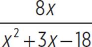 does
does
not equal 0 when the
numerator equals 0
(when x = 0). This
means that g(x) has a
value of 0 at this point.
If the denominator
were also equal to
0, then it would be
undefined, because
0/0 is undefined.

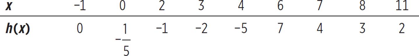
Graph the function h(x) = 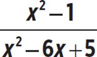 .
.
First, let’s factor both the numerator and the denominator and cancel out any common factors. Remember, when you cancel out a common factor in a rational expression, you must note that x cannot equal the value that would make the factor equal to 0.

In Lesson 2.4, as
we inspected and
simplified rational
expressions, we noted
when an x-value was
excluded from the
domain for making
a rational expression
undefined. As we
look at rational
functions, these
domain restrictions
translate to certain
characteristics of the
function graphs, such
as vertical asymptotes.
h(x) = 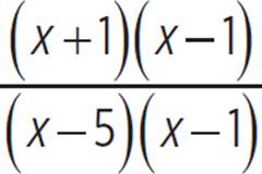
h(x) =  where x ≠ 1
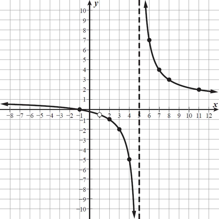
The graph has an x-intercept where x + 1 = 0, or when x = −1. The graph has a y-intercept where x = 0, or at h(0) =  = −1/5. The graph has a vertical asymptote where x − 5 = 0, or when x = 5. We can also create a table of values using the simplified equation, as long as we remember that h(x) is undefined when x = 1.
Here is a graph of h(x) = 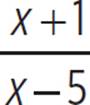 where x ≠ 1.

In Examples 7 and
8, we looked at how
increasing values of
x result in different
levels of increase for
x terms and x2 terms,
while constants remain
unchanged. These
differences of scale
explain why a rational
expression with same
degree polynomials
will tend toward just
the ratio of its highest
degree terms.
Unlike in the previous two examples, this graph does not have a horizontal asymptote at y = 0. Instead, the horizontal asymptote for y = and for y = 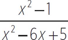 is at y = 1. This is because, for very large values of x, only the x terms to the greatest degree influence the y-values in any significant way. When x is huge, x2 is much greater than 6x, and any x term is definitely much greater than any constant. An x3 term would have much greater influence than any x2 term. When the numerator and denominator are both polynomials to the same degree, then only the highest degree terms have much effect near infinity or negative infinity. This means that for those extreme values of x, the value of
  becomes close to
 ![]() , which simplifies to 1. If one or both of the x2 terms had other coefficients, then the y-values would approach the ratio of those coefficients near x-values of ∞ or −∞.
, which simplifies to 1. If one or both of the x2 terms had other coefficients, then the y-values would approach the ratio of those coefficients near x-values of ∞ or −∞.
When the numerator and denominator polynomials of a rational function are of the same degree, the horizontal asymptote is the line y =  . In Example 9, y = 1/1 = 1.
When the denominator polynomial is of a greater degree than the numerator, the horizontal asymptote is the x-axis, as in the functions in Example 8.
When the numerator polynomial is of a greater degree than the denominator, there is no horizontal asymptote.
When the numerator
polynomial is of a
greater degree than
the denominator, then
as x approaches ∞,
the function value
will approach either
positive or negative ∞,
because the absolute
value of the numerator
will increase much
more quickly than that
of the denominator.
There is a hole in the graph at (1, −1/2) because h(x) = 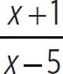 would have a value of −1/2 when x = 1, except that we established that x cannot equal 1.
Try graphing the original rational function, h(x) = using graphing technology. It looks exactly like our graph of h(x) = where x ≠ 1.
Any zero of the denominator in a rational function expression corresponds to a discontinuity in the function’s graph at that x-value. If the zero is also a zero of the numerator, then the discontinuity is a hole in the graph. If the zero is not a common zero for the numerator, then the discontinuity is a vertical asymptote.
We need to acknowledge any discontinuities when describing the domain or range of a function. The domain of h(x) = is all real numbers except for 1 and 5, and the range is all real numbers except for −1/2 and 1.
USING SYSTEMS OF RATIONAL FUNCTIONS TO SOLVE RATIONAL EQUATIONS
Another way to solve a rational equation is to rewrite it as a system of functions, graph the functions, and find the x-values of the points of intersection.

Find all solutions to the following equation.
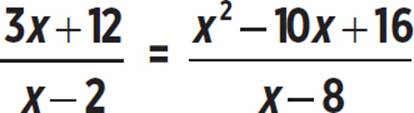
We can create the following system of equations.
f(x) = 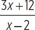
g(x) = 
In Lesson 2.2, we
explored how to use
systems of equations
to solve polynomial
equations. The same
principles apply when
the given equation is a
rational equation. The
x-values of the points
of intersection are the
x-values that make the
original equation true.
The y-intercept occurs
when x = 0. The
x-intercept occurs
when y, or f(x), equals
0, which is when the
numerator, alone, of
the rational expression
equals 0. A vertical
asymptote occurs
when the denominator,
alone, of the rational
expression equals
0. For a rational
function with same
degree polynomials
in the numerator
and denominator,
there is a horizontal
asymptote at the level
of the ratio of the
leading coefficients.
Any point where the graphs of f(x) and g(x) intersect has the same x-value and the same function value [f(x) = g(x)]. The x-values of any points of intersection are the solutions to the equation 
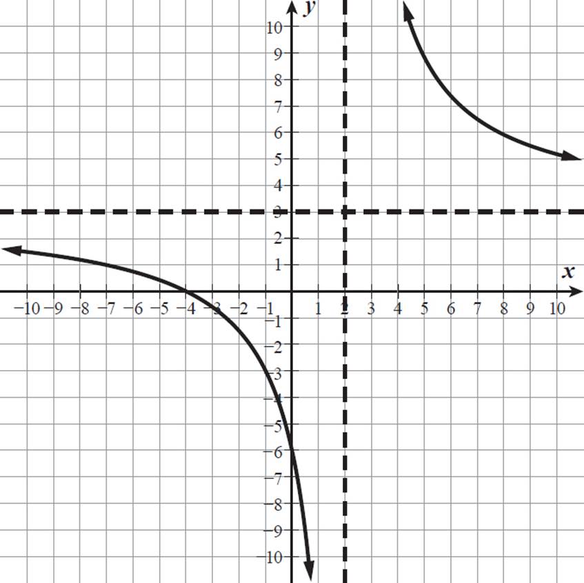
From its equation, we know that the graph of f(x) =  has a y-intercept of −6, an x-intercept of −4, a vertical asymptote at x = 2, and a horizontal asymptote at y = 3. It is always decreasing over each of its continuous sections. Here is its graph.
The function g(x) = 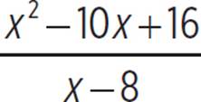 can be rewritten as g(x) =
 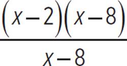 . The numerator and denominator share a common factor of (x − 8), which we can cancel out as long as we also note that x − 8 cannot equal 0. So, g(x) = x − 2 where x ≠ 8. The graph of g(x) is the straight line y = x − 2 with a hole at the point (8, 6). Let’s graph g(x) on the same coordinate grid as f(x).
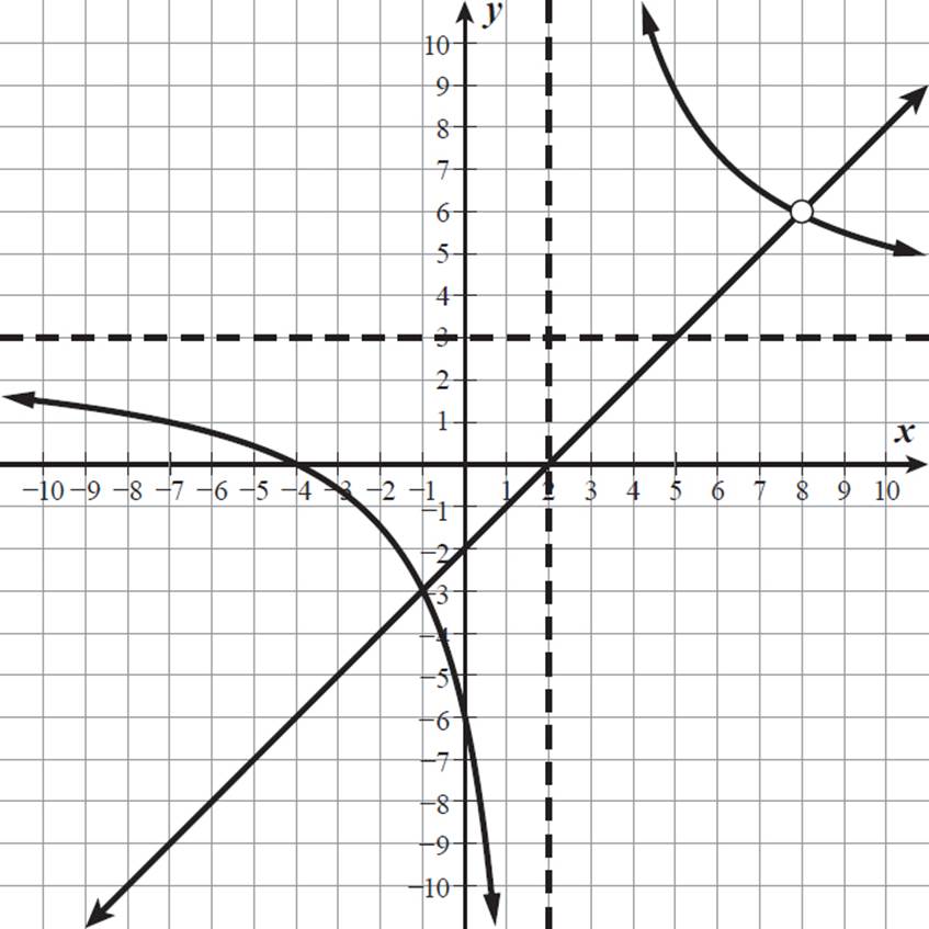
The two functions would have intersected at (8, 6), but there is a hole in the graph of g(x) at this point. Since g(x) does not exist when x = 8, 8 is not a solution for f(x) = g(x). However, the two graphs do intersect at (−1, −3), where there is no discontinuity. The only solution to the original equation is x = −1. Let’s test it, just to make sure.
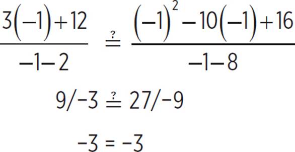
The equation is true, so −1 is the solution for x. Notice that if we had tested 8 in the original equation, it would have produced a denominator of 0 in one fraction, which is undefined.

RATIONAL FUNCTIONS IN THE REAL WORLD
With knowledge of how key features of a function are related to its graph and to its equation, you can compare functions that are described or defined in different ways.

Two music venues each sold out quickly for their respective most popular concerts of the year. Venue A’s most popular concert had a ratio, r, of available seats to unavailable seats given by the equation r =  , where m was the number of minutes since the first ticket was sold. Venue B had a ratio, r, of available seats to unavailable seats m minutes after the first ticket was sold as shown in the function table below. In this table, the m-value of 15 represents the lowest m-value for which r = 0.
|
m |
r |
|
|
0 |
150 |
|
|
1 |
35 |
|
|
3 |
12 |
|
|
8 |
2.8 |
|
|
13 |
0.5 |
|
|
15 |
0 |
Which venue’s seat ratio function has a greater r-intercept, and what does that represent? Which venue’s seat ratio function has a greater m-intercept, and what does that represent?
The r-intercept occurs when m = 0, so the table shows that Venue B has an r-intercept of 150. To find the r-intercept for Venue A, substitute 0 for m and solve for r.
r =  = 200/1 = 200
Venue A has an r-intercept of 200, which is greater than Venue B’s r-intercept of 150. The r-value is the ratio of available seats to unavailable seats m minutes after the first ticket was sold. When m = 0, the very first ticket has just been purchased, so there is only one unavailable seat. At this point, Venue A has a ratio of 200/1, or 200 available seats to 1 unavailable seat, and Venue B has a ratio of 150/1, or 150 available seats to 1 unavailable seat. This means that Venue A must have a total of 201 seats and Venue B must have 151 seats. Venue A has greater seating capacity.
The m-intercept occurs when r = 0. We can see from the table that Venue B has an m-intercept of 15. To find the m-intercept for Venue A, substitute 0 for r and solve for m.
0 = 
0 = 200 − 10m where m ≠ −1/5
10m = 200
m = 20
Time can’t be
negative for this
situation anyway,
so we don’t have to
worry about the fact
that m specifically
can’t equal −1/5.
Venue A has an m-intercept of 20, which is greater than Venue B’s m-intercept of 15. When r = 0, the ratio of available to unavailable seats is zero, so there are no available seats. This is the point at which each venue sells out of tickets to its concert. The variable m represents the minutes since the tickets went on sale. Venue A sold all tickets to its most popular concert in 20 minutes, and Venue B sold all tickets to its most popular concert in 15 minutes. It took Venue A longer to sell out than Venue B.

In Example 11, we were not given the equation for Venue B, but in situations where you are given both of the two equations—or can write them from given information—graphing can be very useful for comparing rational functions.

Karl can sand 4 square meters of wood floor in x hours. Dawn can sand at a rate that is 1 square meter per hour faster than 40% of Karl’s rate. Is one of them definitely faster than the other? If x were defined, how would that answer the question of who sands faster? Explain for which x-values Karl would be faster and for which x-values Dawn would be faster.
First, let’s write functions relating each person’s rate to time. Karl can sand 4 square meters in x hours, so k = 4/x, where k represents Karl’s sanding rate, in square meters per hour. Dawn’s rate is 1 square meter per hour faster than 40% of Karl’s rate, so d = 0.4(4/x) + 1, where d represents Dawn’s sanding rate, in square meters per hour. This equation can be rewritten as the rational function d =  .
.
Let’s graph each of these functions on the same coordinate grid to see how the rates k and d relate to x and to one another.
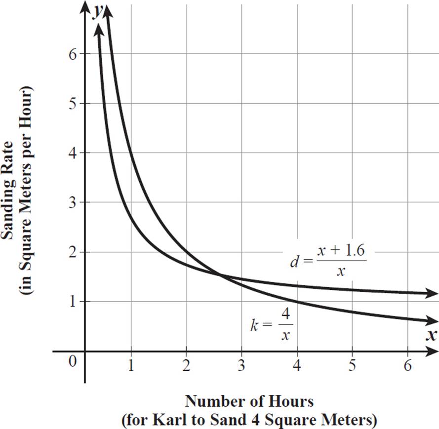
The two functions intersect somewhere between x = 2 and x = 3, so neither Karl nor Dawn is faster for the entire set of x-values. To the left of the point of intersection, k is greater than d, and to the right of it, d is greater than k. Let’s use the equations to find the exact x-value of the point of intersection, where Karl and Dawn would have the same sanding rate.
|
|
Note that x ≠ 0. |
|
4x = x2 + 1.6x |
Cross-multiply. |
|
0 = x2 − 2.4x |
Subtract 4x from both sides. |
|
0 = x(x − 2.4) |
Factor the quadratic. |
|
0 = x or 0 = x − 2.4 |
Set each factor equal to 0. |
Because x ≠ 0, 0 is an extraneous solution, and the only true solution is x = 2.4. Karl and Dawn have the same sanding rate if Karl sands 4 square meters in exactly 2.4 hours.
If x, the number of hours it takes Karl to sand 4 square meters, is defined as less than 2.4 hours, then Karl is the faster sander. If x is defined as greater than 2.4 hours, then Dawn is the faster sander.
