High School Algebra II Unlocked (2016)

Lesson 8.2. Means and Measures of Variability

REVIEW

The mean of a set of data is found by adding the values of all elements in the set and dividing that total by the number of elements in the set.

The interquartile range of a data set is the difference between the upper and lower quartiles of the set.

The lower quartile of a data set is the median of the lower half of the data. It marks the boundary between the lowest 25% of the data and the upper 75%.

The range of a data set is the difference between the maximum value and the minimum value in the set.

The upper quartile of a data set is the median of the upper half of the data. It marks the boundary between the highest 25% of the data and the lower 75%.

Statistics is used not just to measure the mean of a set (or other measures of central tendency), but also the variability of the data in that set, for example, in terms of how far it is from the mean. Two data sets may have the same mean but different variability, even if containing the same number of elements. The sets {9, 10, 10, 10, 10, 11} and {2, 5, 6, 9, 18, 20} each contain six elements and each have a mean of 10, but the data in the second set varies more from the mean.

There are various measures of variability that give you some sense of the dispersion, or spread, of the data. The simplest of these is the range. The set {9, 10, 10, 10, 10, 11} has a range of 2, and the set {2, 5, 6, 9, 18, 20} has a range of 18. Another measure of variability is the interquartile range. The interquartile range of {9, 10, 10, 10, 10, 11} is 0, and the interquartile range of {2, 5, 6, 9, 18, 20} is 13. By only measuring the range of the middle half of the data, the interquartile range provides a better sense of the behavior of data in the set, as compared to the range, which can be greatly affected by very small or large values that are unusual within the set.

Because the lower
quartile marks the
25% point in the data
and the upper quartile
marks the 75% point,
the interquartile
range encompasses
approximately half
of the total elements
in the set. For very
small data sets, the
interquartile range is
not likely to contain
exactly half of the
elements in the set,
but for large data sets,
it contains very close
to, or exactly, 50% of
the elements in the set.

A more precise measure of variability is variance, because it compares each element in the set to the arithmetic mean of the set, which is represented by the Greek letter μ (mu). The variance, σ², is the mean of the squared deviations of all data points from the mean of the data set. In other words, to find the variance, we find the difference between each data point in the set and the mean, square each of those differences, and then find the mean of the squares.

The formula for variance is: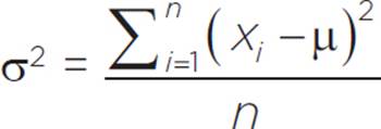
,
where x_i represents the ith element of the data set, n represents the number of elements in the set, and μ represents the mean of the set.

The purpose of
squaring the
differences is to
eliminate the variation
between positive
and negative values,
and focus instead on
the distance of each
element from the
mean of the set.

For the set {9, 10, 10, 10, 10, 11}, the variance is given by , which simplifies to 1/3, or 0.3. Variance is always expressed in square units for data points in units, because it is an average of the squares of deviations.

For the set {2, 5, 6, 9, 18, 20}, the variance is given by , which is equal to 45 square units. The variance for this set is much greater than the variance for the first set.

Often, a statistician is analyzing data for a sample from a target population, not data for the entire target population. In this case, we should use the formula for estimated variance, s². The estimated variance is, confusingly, sometimes called sample variance, but it is an estimate of the variance of the entire population based on data from a sample.

The formula for estimated variance is: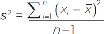
,
where x_i represents the ith element of the sample data set, n represents the number of elements in the sample set, and x represents the mean of the sample data set.

Notice that, in the estimated variance formula, the sum of squares is divided by (n − 1) instead of n. The smaller denominator produces a larger variance value, to account for the possibility that data for the target population varies more than what is shown within the sample set.

If the set {2, 5, 6, 9, 18, 20} is a sample from a larger population that we are studying, then we would estimate the variance of the population using the estimated variance formula with data from this sample set.

Simplified, the estimated variance for the population, based on the given sample set, is 54 square units.

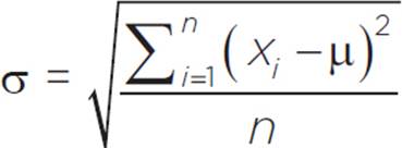
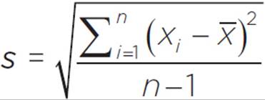
If we take the square root of the variance of a data set, the result is the standard deviation of the data set, indicated by the Greek letter σ (sigma). Likewise, the square root of the estimated variance is the estimated standard deviation, also sometimes called the sample standard deviation. The estimated standard deviation is the estimate of the standard deviation for the entire population based on data from a sample.

The Greek letter σ that
we use to represent
standard deviation is a
lower-case sigma. The
upper-case sigma, Σ,
represents a sum, as
used in the standard
deviation formula.

Standard Deviation:

Estimated Standard Deviation:

The heights of the members of the high school girls’ volleyball team are {5.2, 5.4, 5.4, 5.5, 5.5, 5.5, 5.7, 5.8, 6.0, 6.0}, in feet. The heights, in feet, of the members of the high school boys’ basketball team are {5.6, 5.9, 5.9, 6.0, 6.0, 6.1, 6.1, 6.3, 6.4, 6.6, 6.7, 6.8}. Compare the means and standard deviations for the two teams. What do these indicate about the heights of players on each of these two teams?

To calculate the mean height of a player, add all heights for that team and divide the total by the number of players on the team. Notice that the number of players is different for the two teams: 10 girls on the volleyball team and 12 boys on the basketball team.

Girls’ volleyball team:

μ = 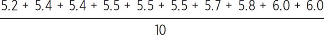= 56/10 = 5.6

Boys’ basketball team:

μ = = 74.4/12 = 6.2

For each team, the data given is for the entire population, so we are calculating the actual standard deviation, not an estimated standard deviation. Use the formula σ = .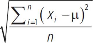

Girls’ volleyball team: σ =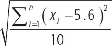

Boys’ basketball team: σ =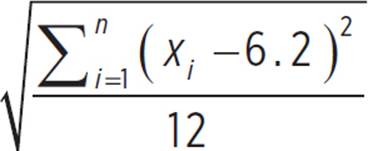

Now is a good time to use a calculator or computer program that will calculate the standard deviation for you. For the girls’ volleyball team, the population variance is 0.064, and the population standard deviation is about 0.25. For the boys’ basketball team, the population variance is 0.12167, and the population standard deviation is about 0.35.

Here is how you may see mean and standard deviation on the SAT.

Barbara’s company had record profits last year. To thank her employees for their hard work, she divided a portion of the profits equally among all of her employees, so each employee received a bonus of $5,000. What effect does this bonus have on the mean and standard deviation of the employees’ incomes for that year?

A) It would have no effect on the mean but would increase the standard deviation.

B) It would increase the mean but decrease the standard deviation.

C) It would increase the mean but have no effect on the standard deviation.

D) It would increase the mean and the standard deviation.

The mean height of a player on the boys’ basketball team, 6.2 feet, is 0.6 foot greater than the mean height of a player on the girls’ volleyball team, 5.6 feet. The heights of players on the boys’ basketball team have a greater standard deviation, 0.35 foot, than those of players on the girls’ volleyball team, 0.25 foot. In other words, the boys’ basketball team members tended to be taller than the girls’ volleyball team members, and there was more variation in their heights (they were more spread out from the mean).