High School Algebra II Unlocked (2016)

Lesson 8.5. Sample Proportions and Sampling Distribution

REVIEW

A bimodal distribution is a data distribution that has two local maximums. As a distribution curve, it has two humps, in contrast to a normal distribution, which has just one.

A Bernoulli trial is a random experiment that has exactly two possible outcomes in its sample space (called “successes” and “failures”), with the same probability of success for every time the experiment is repeated. A repeated coin toss is one example of a Bernoulli trial. Repeatedly drawing a marble from a bag of 7 purple and 3 green marbles, with replacement of the drawn marble each time, is also a Bernoulli trial.

If we wanted to determine the percentage of voters who will vote to re-elect the current president, we might poll a sample of the population, because we cannot poll every voter in the country. A sample proportion is the ratio of successes to total number of experiments or observations in the sample. If we polled 200 voters, and 72 of them said they would vote for the incumbent president, then the sample proportion is 72/200, or 0.36.

If you did not put the
marble back in the bag
after drawing, the total
number of marbles
in the bag and the
number of marbles of
one color would both
decrease, resulting in
a different probability
for the next draw.

Sample proportion, , is given by = x/n, where x = the number of successes and n = the number of Bernoulli trials or number of observations in the sample.

For large values of n (large sample sizes), the sample proportions of Bernoulli trials follow an approximately normal distribution. A good rule of thumb is that the distribution of will be normal if the sample is large enough to include at least 10 successes and at least 10 failures.

Ideally, these numbers of successes and failures are based on the “true” percentages (population proportions) applied to the sample size. However, in the case that the population proportion, p, is unknown, we use the sample proportion, , i.e., the actual number of successes and failures in the sample.

If samples are repeatedly drawn from a population (or a Bernoulli trial is repeatedly performed), with np ≥ 10 and n(p − 1) ≥ 10, then the sample proportions are approximately normally distributed.

The idea is that there is some underlying “true” percentage (the percentage of total voters who will vote to re-elect the incumbent president; the 50% probability of a coin landing on heads), and repeated trial/sample percentages will be normally distributed in relation to this percentage. In other words, p = μ for the normal distribution curve of sample proportions.

When the population size is at least 20 times as large as the sample size, then the standard deviation of the sampling distribution (a normal distribution of sample proportions) is given by the formula 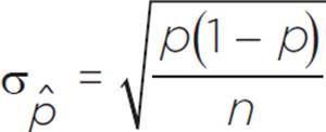, where p is the population proportion and n is the sample size.

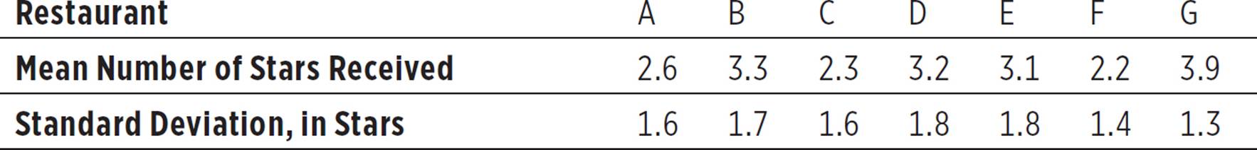
Patra took restaurant rating data from a website that allows users to rate restaurants with a star system, with the lowest rating being one star and the highest rating being five stars. She took randomly chosen samples of 20 review ratings for each of seven restaurants and calculated the mean and standard deviation for each data set, as shown in the table below.

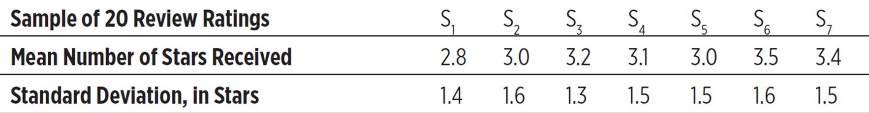
She then took random samplings of seven sets of 20 reviews from the full set of 5000 reviews on the website. The means and standard deviations of these sets are shown below.

(a) If a restaurant received the same number of each level of review within a set of 20 reviews, what would be the mean and standard deviation for the number of stars received per review? How is Patra’s data different?

(b) Based on a theoretical probability of each star rating being equally likely, what would be the expected number of times a rating of 3 stars would appear in any 20-review sample set? What would be the standard deviation for the sampling distribution of 3-star ratings, assuming normal distribution? Suppose Patra recorded the number of 3-star ratings in each of her 14 data sets, as follows: {0, 0, 0, 1, 1, 1, 1, 1, 1, 2, 2, 2, 3, 3}. What might the probability distribution graph for actual ratings, in stars, look like? What is a possible explanation for this difference in sampling distribution?

(a) If a restaurant received the same number of each level of review within a set of 20 reviews, then it would receive the following numbers of stars: {1, 1, 1, 1, 2, 2, 2, 2, 3, 3, 3, 3, 4, 4, 4, 4, 5, 5, 5, 5}. The mean for this set is 3, and the standard deviation is 1.45. Patra’s sets have similar means (the average of all the means is about 3), but higher standard deviations in most cases. This means there is more variability in Patra’s data.

(b) If each star rating were equally likely, then a rating of 3 stars would have a probability of 1/5. In a 20-review sample set, there would be about 1/5 (20) = 4 reviews of 3 stars.

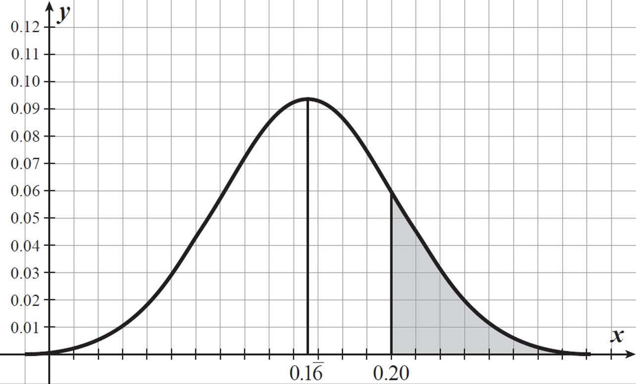
1/5 (5000) ≥ 10 and 4/5 (5000) ≥ 10, so we can determine a normal distribution based on this theoretical probability. The standard deviation of the sampling distribution (in terms of sample proportions) would be 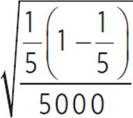≈ 0.0057. So, the probability distribution for a result of 3 stars would have a mean of 1/5 and a σ of 0.0057. We can convert this to number of 3-star ratings per 20-rating sample by multiplying by 20. The probability distribution for number of 3-star ratings per 20-rating set would have a mean of 4 reviews and a standard deviation of 0.11 review.

The actual number of 3-star ratings per 20-rating set are much lower. All of them are fewer than 4 reviews. With a σ of 0.11 review, the theoretical probability set for number of 3-star ratings per sample set should have 99.7% of outcomes within 3(0.11) review of the mean. In other words, 99.7% of outcomes should include between 3.67 and 4.33 stars. The actual number of 3-star ratings consistently fall in the other 0.3% probability space. This means that Patra’s results are not at all consistent with a normal distribution of ratings.

With very few 3-star ratings but a mean of around 3 stars per review, and a large standard deviation, Patra’s data consists of mostly very high ratings and very low ratings, so it has a bimodal probability distribution. The actual probability distribution of individual ratings, in terms of number of stars, is a discrete probability set and might look something like this.

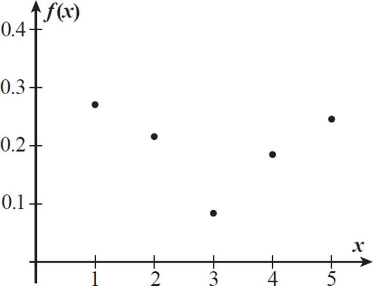
One possible explanation for the star rating data is that there is a voluntary bias. The ratings are given voluntarily, and the people who post those ratings on the website tend to be people who feel very strongly about a restaurant, whether positively or negatively. People who consider the restaurant average (3 stars) may not be as inspired to post a review.

Elton and Robin are playing a game in which they roll two dice and record the sum. Out of 100 sums recorded, there were 20 sums of 10 or greater. Elton thinks this is unusually high. Use the sampling distribution for this series of Bernoulli trials to determine the probability of rolling a sum of 10 or greater 20 out of 100 times.

Because the probabilities of dice follow uniform distributions, we can find the true population proportion: the theoretical probability of rolling a sum of 10 or greater. There are a total of 6 ⋅ 6 = 36 possible outcomes for rolling two dice, and 6 of those outcomes result in a sum of 10 or greater (4 + 6, 5 + 5, 5 + 6, 6 + 4, 6 + 5, and 6 + 6), so the theoretical probability of rolling a sum greater than or equal to 10 is 6/36, or 1/6.

In each sum, the first
number represents the
value on die number
1 and the second
number represents the
value on die number
2. We must count
both 4 + 6 and 6 + 4
as distinct ways of
rolling a sum of 10.

Let’s test if this situation is eligible for fitting to a normal distribution curve.

np = 100 ⋅ 1/6 = 16.6
n(1 − p) = 100 ⋅ 5/6 = 83.3

Both of these projected success and failure numbers are greater than 10, so the distribution of the sample proportions is approximately normal.

Using p = 1/6 and n = 100, we can calculate the standard deviation for the sampling distribution.

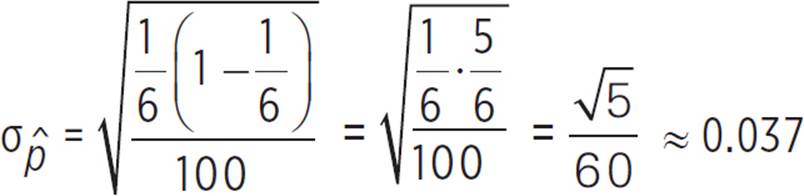
The population proportion, or theoretical probability, of 1/6, or 0.16, is the mean for the sampling distribution, and the standard deviation is 0.037.

The sample proportion (the experimental probability) in this case is 20/100, or 1/5, because Elton and Robin rolled a sum of at least 10 in 20 of their 100 tries. We want to compare this of 1/5, or 0.2, to the mean of 0.16, in terms of a standard deviation of 0.037.

The difference between and p is 0.2 − 0.16 = 0.03. This is an absolute difference. We need to convert it to be in terms of numbers of standard deviations.

0.03/0.037 ≈ 0.9

The mean for the
sampling distribution
is also called the
expected value. In this
trial, you theoretically
expect to have a
1/6 success rate.

The sample proportion, 0.2, is 0.9 of a standard deviation to the right of the mean, 0.16.

The value 1σ to the right of the mean is 0.16 + 0.037 = 0.204. The percentage of area under the curve to the right of this value is 1 − 0.84 = 0.16. This means that in 16% of trials (each trial a set of 100 rolls of the dice), the proportions of successes (getting a sum of 10 or greater) to number of dice throws is 0.204 or more. Elton and Robin’s sample proportion, 0.2, is to the left of 0.204, so the above statement definitely also applies to a sample proportion of 0.2. In other words, you can expect a 1/5 success rate in about 16% of 100-toss trials.

Notice that, because
our random variable
changed, the
standard deviation
also changed. For
the distribution
of trial success
numbers, the standard
deviation is 3.7.

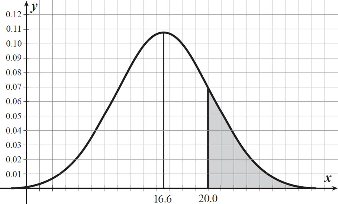
It might be easier to interpret a distribution of trial results (number of times a sum of 10 or greater is rolled per trial) instead of a distribution of sample proportions. The number of expected successes, according to the theoretical probability, is np: 100 ⋅ 1/6 = 16.6. The actual number of successes for sample proportion is n. It is the n that follows a normal distribution with a mean of np in the graph below, showing probability distribution of sample/trial results.

Because the sample
size is 100 for each
trial, the number of
successful trial results
looks very similar to
the sample proportion
(percentage) for
successful trial results.
Multiplying each
proportion value by
100 simply moves
the decimal point two
places to the right.

This graph makes it more apparent that a result of 20 or more successes occurs in 16% of trials (each trial being 100 tosses of two dice). This is not such an unusual occurrence.

A typical cutoff for determining a result to be highly unusual is subjective but is often when that result occurs only 5% of the time or less, under a normal distribution.