Master AP Calculus AB & BC
Part II. AP CALCULUS AB & BC REVIEW
CHAPTER 11. Sequences and Series (BC Topics Only)
TAYLOR AND MACLAURIN SERIES
NOTE. Just like power series, Taylor series are stressed very heavily on the AP test.
At the end of the power series section, we saw that a function can be defined using a power series. Taylor series are specific forms of the power series that are used to approximate function values. For example, you know cos π and cos π/2 by heart, but if asked to evaluate cos 1/2, you’d probably be stumped. (Arccos 1/2 is very easy; that is π/3, but cos 1/2 is rough.) We can create a very simple Taylor series that will approximate cos 1/2 very nicely. We will create a power series centered around a very easily obtained value of cosine that is also close to 1/2. The best choice is c = 0, since 0 is close to 1/2 and cos 0 is easy to evaluate; cos 0 = 1.
NOTE. Remember, the notation f(n)(x) means the nth derivative of f(x).
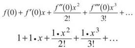
Taylor series for f(x) centered about x = c: 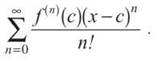
![]()
Most of the time, you will not use an infinite series to approximate function values. Instead, you will use only a finite number of the series’ terms. In these cases, the Taylor series is often called a Taylor polynomial of degree n (where n is the highest power of the resulting polynomial). A Maclaurin series is the specific case of a Taylor series that is centered at c = 0, resulting in the simpler-looking series 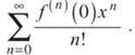
![]()
TIP. All Maclaurin series are also Taylor series; they are just special Taylor series.
Example 15: Use a fourth-degree Taylor polynomial of order (degree) 4 centered at 0 to approximate cos (1/2).
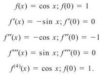
Solution: Since this Taylor series is centered at c = 0, it is actually a Maclaurin series. We will have to use the Maclaurin series expansion up to n = 4, since the requested degree is 4. In order to find the series, we will have to find f(0), f'(0), f"(0), f'"(0), and f(4)(x):
To get the Maclaurin polynomial, plug these into the Maclaurin formula and stop when n = 4:
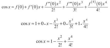
The resulting polynomial will give you the approximate value of cos x. To find the approximate value of cos 1/2, plug 1/2 in for x:
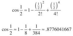
The actual value for cos 1/2 (according to the calculator) is .8775825619, so the approximation wasn’t too shabby at all. Just like Riemann sums, the accuracy of your prediction will increase as you increase the number of terms in your Taylor polynomial; in other words, the greater the n, the more accurate the result. Below, the graph of y = cos x is compared with the graphs of three Maclaurin polynomials for cos x centered about 0.

A couple of things are clear from the graphs. First of all, the greater the degree of the polynomial, the closer its graph is to the graph of cos x. However, none of the approximations are very good for approximating values far away from x = 0. If you need to approximate other values, you will have to use a Taylor polynomial centered about a different value. For example, to estimate cos (3.2), you might use a Taylor series centered about c = π, since π is close to 3.2.
NOTE. A Taylor series is guaranteed to give the exact function value only for x = c, the value around which the series is centered. All other values will likely be approximations.
Although it wasn’t too difficult to come up with the Maclaurin polynomial for cos x, you shouldn’t have to construct it like that on the AP test. It is one of four functions for which you should have the Maclaurin expansions memorized—doing so will save you much-needed time.
Maclaurin Series to Memorize
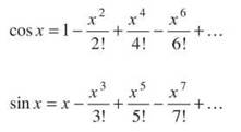
Not all of the series on the AP test will be based on these four functions, but most of them will. Any other series can be constructed using the method of Example 15.
ALERT! Each of the Maclaurin series listed will converge on (-∞,∞), except for ![]() That series has an interval of convergence of (-1,1) and will not work well for x’s outside that interval.
That series has an interval of convergence of (-1,1) and will not work well for x’s outside that interval.
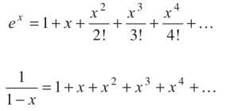
Example 16: Derive the Maclaurin series for sin x from the Maclaurin series for cos x.
Solution: We know that ∫cos x dx = sin x. Taylor series act just like their parent functions; if you integrate each term of the cos x Maclaurin series, you will end up with the Maclaurin series for sin x. This is not only useful for impressing your friends, however.
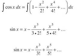
The resulting series is exactly the one for sin x that you are to memorize.
ALERT! Even though the sin x series is written ![]() the next term in the series, -x7/7!, is still negative. The series still alternates; it’s just common notation to write a “+” at the end of an infinite series, regard less of the sign of the next term.
the next term in the series, -x7/7!, is still negative. The series still alternates; it’s just common notation to write a “+” at the end of an infinite series, regard less of the sign of the next term.
Example 17: Determine a power series for sin x2.
Solution: Besides acting like their parent functions, Taylor series are also handy because they are very flexible. We already know the Maclaurin series for sin x (and Taylor and Maclaurin series are just special power series anyway). To find the series for x2, just plug x2 in for x. That’s all there is to it.
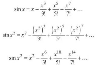
If the question had asked you to find a series for sin (2x + 3), all you would do is plug (2x + 3) in for x. Simple!
Like alternating series, there is a way to tell how accurately your Taylor polynomial approximates the actual function value: you use something called the Lagrange remainder or Lagrange error bound. It is the trickiest part of Taylor series.
Lagrange Remainder: If you use a Taylor polynomial of degree n centered about c to approximate the value x, then the actual function value falls within the error bound
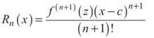
where z is some number between x and c.
Translation: Similar to alternating series, the error bound is given by the next term in the series, n + 1. The only tricky part is that you evaluate f(n+1), the (n + 1)th derivative, at z, not c. What the heck is z, you ask? It is the number that makes f(n+1)(z) as large as it can be. This error bound is supposed to tell you how far off you are from the real number, so we want to assume the worst. We want the error bound to represent the largest possible error. In practice, picking z is relatively easy—really, you’ll see.
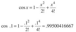
Example 18: Approximate cos (A) using a fourth-degree Maclaurin polynomial, and find the associated Lagrange remainder.
Solution: We already know the fourth-degree Maclaurin polynomial for cosine, so plug .1 in for x to get the approximation:
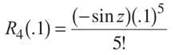
The associated Lagrange remainder for n = 4 (denoted R4(x)) is
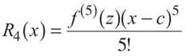
The fifth derivative of cos x is —sin x, so f(5)(z) = —sin z. Now, plug in x = .1 and c = 0 to get
TIP. f(n+1)(z) will often have a value of 1 on AP problems, making the Lagrange remainder simply the value of the next term in the series, as it turned out to be in Example 18.
We need —sin z to be as large as it can possibly be. The largest value of —sin x is 1, since —sin x, like sin x, has a range of [—1,1]. By assuming —sin z is the largest possible value, we are creating the largest possible error; so, plug in 1 for —sin z. The actual remainder will be less than this largest possible value.
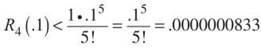
Therefore, our approximation of .99500416667 is off by no more than .0000000833. In fact, it is only off by .0000000014.
EXERCISE 4
Directions: Solve each of the following problems. Decide which is the best of the choices given and indicate your responses in the book.
YOU MAY USE A GRAPHING CALCULATOR FOR PROBLEMS 3 AND 4.
1. (a) Verify that the Maclaurin expansion for ![]()
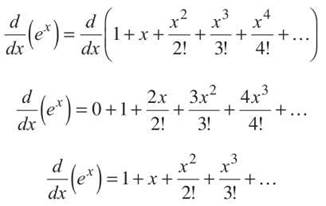
(b) Show that the Maclaurin series for ex (like the function it represents) is its own derivative.
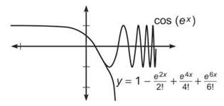
2. (a) Create a Maclaurin series for g(x) = cos (ex).
(b) Use a sixth-degree Mauclaurin series to approximate cos e2.
(c) Explain why the approximation in 2(b) is so horrid.
3. Estimate the value of √1.3 using the third-degree Taylor polynomial for y = √x centered about x = 1.
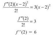
4. Let P(x) = 4 — (x — 2) + 3(x — 2)2 — 5(x — 2)3 be a Taylor polynomial of degree 3 for f(x) centered about 2.
(a) What is f"(2)?
(b) Use a second-degree Taylor polynomial to approximate f'(2.1).
ANSWERS AND EXPLANATIONS
1. (a) The Maclaurin series is 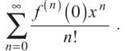 To write out the expansion, we’ll need f(0), f'(0), f"(0), etc.
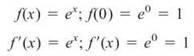
In fact, each derivative of ex is ex, and each derivative’s resulting value at x = 0 will be 1. Therefore, the series is
which is the expansion we all know and love.
(b) Find the derivative of each term of the series separately:
(a) You already know the Maclaurin series for cos x, so just plug ex in for each x:
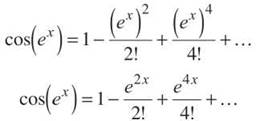
(b) Based on your work for 2(a), the sixth-degree Maclaurin polynomial for cos x is
![]()
To approximate cos e2, plug 2 in for x:
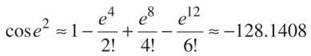
Whoa, how can cosine have a value lower than —1? Yikes!
(c) Remember that a Taylor series is only accurate around the value at which it is centered. Because this is a Maclaurin series, it’s centered at c = 0. Using this approximation to evaluate cos (e2) is irresponsible, since e2 ≥ 7.389, which is nowhere close to c = 0. As you can see from the graph of y = cos (ex) and the Maclaurin series in 2(b), the graphs are nowhere close to each other as you get farther away from x = 0.
3. To find the third-degree Taylor polynomial for f(x) centered at c = 1, we’ll need the value of the first three derivatives of f evaluated at 1; these are required by the formula.
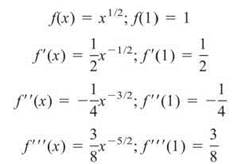
Therefore, the Taylor polynomial is
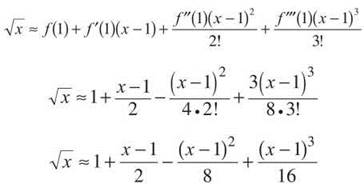
Finally, plug in x = 1.3 to get the approximation of 1.1404375, which is relatively close to the actual value of 1.140175.
4. (a) We know that the squared term in any Taylor polynomial is given by ![]() In this problem, that term should be
In this problem, that term should be ![]() In the actual expansion, the squared term is 3(x — 2)2. Therefore,
In the actual expansion, the squared term is 3(x — 2)2. Therefore,
(b) This question asks you to approximate the value of the derivative of f. Since a Taylor series acts like its parent function, you can approximate f'(x) by taking the derivative of each term:
![]()
This is the second-degree polynomial to which the problem is alluding. You can use it to find your approximation since 2.1 is close to 2, the value at which the series is centered:
![]()
Isn’t that bizarre? We don’t even know the function that P approximates, but we can still approximate its derivative.