5 Steps to a 5 AP Calculus AB & BC, 2012-2013 Edition (2011)
STEP 4. Review the Knowledge You Need to Score High
Chapter 13. More Applications of Definite Integrals
IN THIS CHAPTER
Summary: In this chapter, you will learn to solve problems using a definite integral as accumulated change. These problems include distance-traveled problems, temperature problems, and growth problems. You will also learn to work with slope fields, solve differential and logistic equations, and apply Euler’s Method to approximate the value of a function at a specific value. Please note that logistic equations and Euler’s Method are tested on the AP Calculus BC exam only.

Key Ideas
![]() Average Value of a Function
Average Value of a Function
![]() Mean Value Theorem for Integrals
Mean Value Theorem for Integrals
![]() Distance Traveled Problems
Distance Traveled Problems
![]() Definite Integral as Accumulated Change
Definite Integral as Accumulated Change
![]() Differential Equations
Differential Equations
![]() Slope Fields
Slope Fields
![]() Logistic Differential Equations
Logistic Differential Equations
![]() Euler’s Method
Euler’s Method
13.1 Average Value of a Function
Main Concepts: Mean Value Theorem for Integrals, Average Value of a Function on [a, b]
Mean Value Theorem for Integrals
If f is continuous on [a, b], then there exists a number c in [a, b] such that 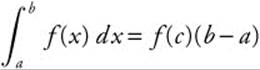 . (See Figure 13.1-1.)
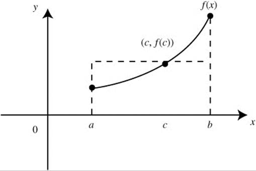
Figure 13.1-1
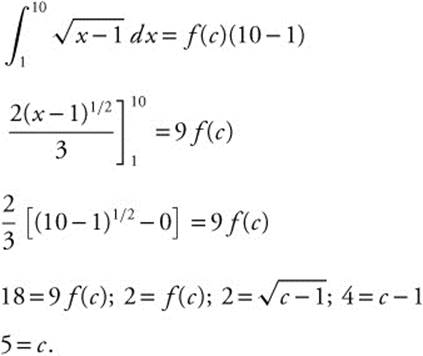
Example 1
Given ![]() , verify the hypotheses of the Mean Value Theorem for Integrals for f on [1, 10] and find the value of c as indicated in the theorem.
, verify the hypotheses of the Mean Value Theorem for Integrals for f on [1, 10] and find the value of c as indicated in the theorem.
The function f is continuous for x ≥ 1, thus:
Example 2
Given f(x) = x2, verify the hypotheses of the Mean Value Theorem for Integrals for f on [0, 6] and find the value of c as indicated in the theorem.
Since f is a polynomial, it is continuous and differentiable everywhere,
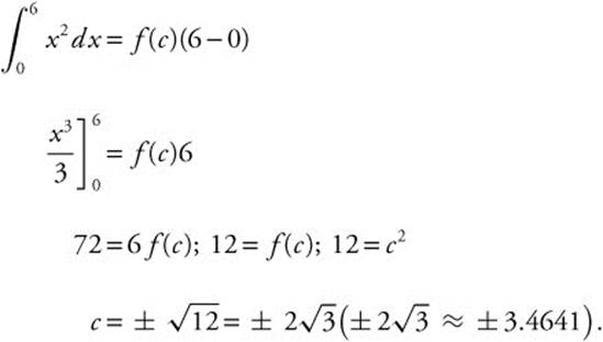
Since only ![]() is in the interval [0, 6],
is in the interval [0, 6], ![]() .
.

• Remember: if f′ is decreasing, then f″ < 0 and the graph of f is concave downward.
Average Value of a Function on [a, b]
Average Value of a Function on an Interval
If f is a continuous function on [a, b], then the Average Value of f on 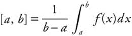 .
.
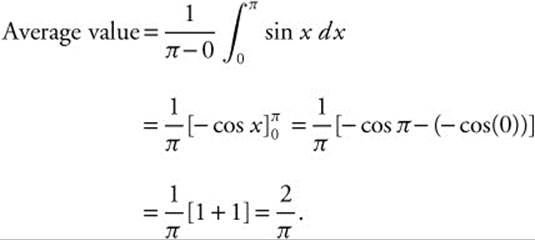
Example 1
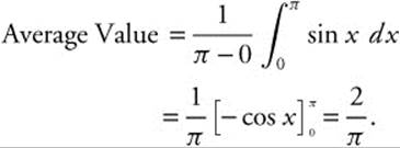
Find the average value of y = sin x between x = 0 and x = π.
Example 2
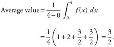
The graph of a function f is shown in Figure 13.1-2. Find the average value of f on [0, 4].
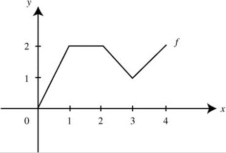
Figure 13.1-2
Example 3
The velocity of a particle moving on a line is v(t) = 3t2 − 18t + 24. Find the average velocity from t = 1 to t = 3.
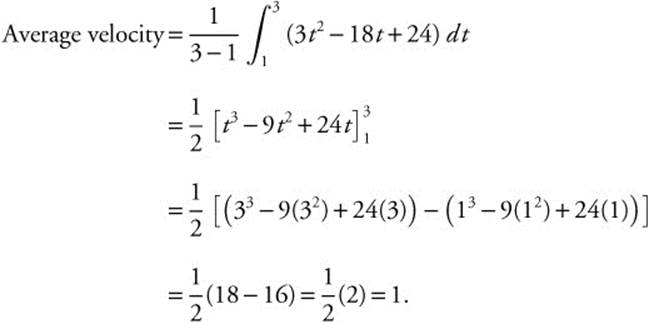
Note: The average velocity for t = 1 to t = 3 is ![]() , which is equivalent to the computations above.
, which is equivalent to the computations above.
13.2 Distance Traveled Problems
Summary of Formulas
Position Function: s(t); 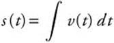 .
.
Velocity: ![]() ;
; 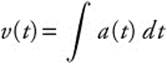 .
.
Acceleration: ![]() .
.
Speed: |v(t)|.
Displacement from t1 to 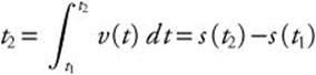 .
.
Total Distance Traveled from t1 to 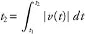 .
.
Example 1
See Figure 13.2-1.
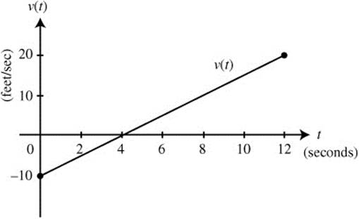
Figure 13.2-1
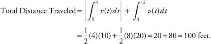
The graph of the velocity function of a moving particle is shown in Figure 13.2-1. What is the total distance traveled by the particle during 0 ≤ t ≤ 12?
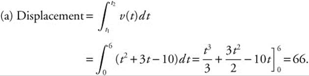
Example 2
The velocity function of a moving particle on a coordinate line is v(t) = t2 + 3t − 10 for 0 ≤ t ≤ 6. Find (a) the displacement by the particle during 0 ≤ t ≤ 6, and (b) the total distance traveled during 0 ≤ t ≤ 6.
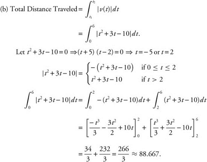
The total distance traveled by the particle is ![]() or approximately 88.667.
or approximately 88.667.
Example 3
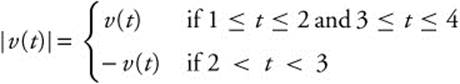
The velocity function of a moving particle on a coordinate line is v(t) = t3 − 6t2 + 11t − 6. Using a calculator, find (a) the displacement by the particle during 1 ≤ t ≤ 4, and (b) the total distance traveled by the particle during 1 ≤ t ≤ 4.
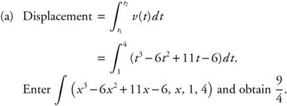
(b) Total Distance Traveled 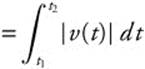 .
.
Enter y1 = x^3 − 6x^2 + 11x − 6 and use the [Zero] function to obtain x-intercepts at x = 1, 2, 3.
Total Distance Traveled 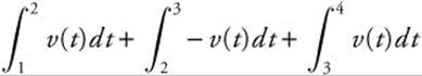 .
.
Enter  and obtain
 ![]() .
.
Enter  and obtain
 ![]() .
.
Enter  and obtain
 ![]() .
.
Thus, total distance traveled is  .
.
Example 4
The acceleration function of a moving particle on a coordinate line is a(t) = − 4 and v0 = 12 for 0 ≤ t ≤ 8. Find the total distance traveled by the particle during 0 ≤ t ≤ 8.
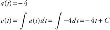
Since v0 = 12 ⇒ − 4(0) + C = 12 or C = 12.
Thus, v(t) = − 4t + 12.
Total Distance Traveled 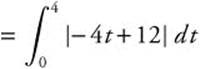 .
.
Let − 4t + 12 = 0 ⇒ t = 3.
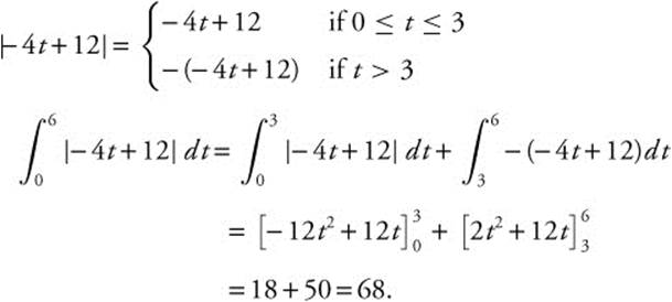
Total distance traveled by the particle is 68.
Example 5
The velocity function of a moving particle on a coordinate line is v(t) = 3 cos(2t) for 0 ≤ t ≤ 2π. Using a calculator:
(a) Determine when the particle is moving to the right.
(b) Determine when the particle stops.
(c) The total distance traveled by the particle during 0 ≤ t ≤ 2π.
Solution:
(a) The particle is moving to the right when v(t) > 0.
Enter y 1 = 3 cos(2x). Obtain y1 = 0 when ![]() ,
, ![]() ,
, ![]() , and
, and ![]() .
.
The particle is moving to the right when: ![]() ,
, ![]() ,
, ![]() .
.
(b) The particle stops when v(t) = 0.
Thus the particle stops at ![]() ,
, ![]() ,
, ![]() , and
, and ![]() .
.
(c) Total distance traveled 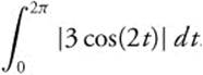 .
.
Enter  and obtain 12. The total distance traveled by the particle is 12.
13.3 Definite Integral as Accumulated Change
Main Concepts:
Business Problems, Temperature Problem, Leakage Problem, Growth Problem
Business Problems
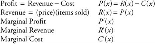
P′(x), R′(x), and C′(x) are the instantaneous rates of change of profit, revenue, and cost, respectively.
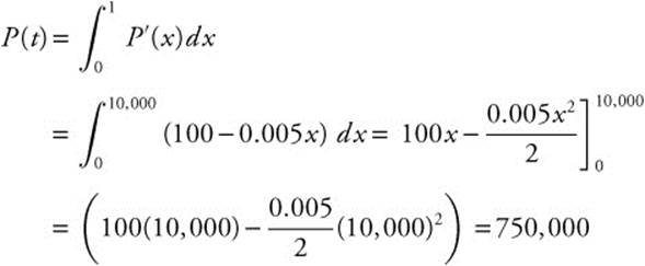
Example 1
The marginal profit of manufacturing and selling a certain drug is P′(x) = 100 − 0.005x.
How much profit should the company expect if it sells 10,000 units of this drug?
• If f″(a) = 0, f may or may not have a point of inflection at x = a, e.g., as in the function f(x) = x4, f″(0) = 0 but at x = 0, f has an absolute minimum.
Example 2
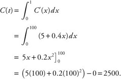
If the marginal cost of producing x units of a commodity is C′(x) = 5 + 0.4x, find (a) the marginal cost when x = 50;
(b) the cost of producing the first 100 units.
Solution:
(a) Marginal cost at x = 50:
C′(50) = 5 + 0.4(50) = 5 + 20 = 25.
(b) Cost of producing 100 units:
Temperature Problem
Example
On a certain day, the changes in the temperature in a greenhouse beginning at 12 noon are represented by ![]() degrees Fahrenheit, where t is the number of hours elapsed after 12 noon. If at 12 noon, the temperature is 95°F, find the temperature in the greenhouse at 5 p.m.
degrees Fahrenheit, where t is the number of hours elapsed after 12 noon. If at 12 noon, the temperature is 95°F, find the temperature in the greenhouse at 5 p.m.
Let F(t) represent the temperature of the greenhouse.
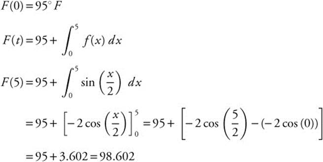
The temperature in the greenhouse at 5 p.m. is 98.602°F.
Leakage Problems
Example
Water is leaking from a faucet at the rate of l (t) = 10e−0.5t gallons per hour, where t is measured in hours. How many gallons of water will have leaked from the faucet after a 24 hour period?
Let L(x) represent the number of gallons that have leaked after x hours.
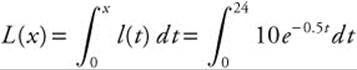
Using your calculator, enter ![]() (10e^(− 0.5x), x, 0, 24) and obtain 19.9999. Thus, the number of gallons of water that have leaked after x hours is approximately 20 gallons.
(10e^(− 0.5x), x, 0, 24) and obtain 19.9999. Thus, the number of gallons of water that have leaked after x hours is approximately 20 gallons.
• You are permitted to use the following 4 built-in capabilities of your calculator to obtain an answer; plotting the graph of a function, finding the zeros of a function, finding the numerical derivative of a function, and evaluating a definite integral. All other capabilities of your calculator can only be used to check your answer. For example, you may not use the built-in [Inflection] function of your calculator to find points of inflection. You must use calculus using derivatives and showing change of concavity.
Growth Problem
Example
On a farm, the animal population is increasing at a rate which can be approximately represented by g(t) = 20 + 50 ln(2 + t), where t is measured in years. How much will the animal population increase to the nearest tens between the third and fifth years?
Let G(x) be the increase in animal population after x years.
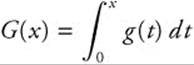
Thus, the population increase between the third and fifth years
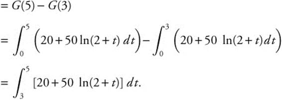
Enter 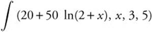 and obtain 218.709.
Thus the animal population will increase by approximately 220 between the 3rd and 5th years.
13.4 Differential Equations
Main Concepts:
Exponential Growth/Decay Problems, Separable Differential Equations
Exponential Growth/Decay Problems
1. If ![]() , then the rate of change of y is proportional to y.
, then the rate of change of y is proportional to y.
2. If y is a differentiable function of t with ![]() , then y(t) = y0ekt; where y0 is initial value of y and k is constant. If k > 0, then k is a growth constant and if k < 0, then k is the decay constant.
, then y(t) = y0ekt; where y0 is initial value of y and k is constant. If k > 0, then k is a growth constant and if k < 0, then k is the decay constant.
Example 1—Population Growth
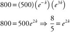
If the amount of bacteria in a culture at any time increases at a rate proportional to the amount of bacteria present and there are 500 bacteria after one day and 800 bacteria after the third day:
(a) approximately how many bacteria are there initially, and
(b) approximately how many bacteria are there after 4 days?
Solution:
(a) Since the rate of increase is proportional to the amount of bacteria present, then:
![]() where y is the amount of bacteria at any time.
where y is the amount of bacteria at any time.
Therefore, this is an exponential growth/decay model: y(t) = y0ekt.
Step 1. y(1) = 500 and y(3) = 800
500 = y0ek and 800 = y0e3k
Step 2. ![]()
Substitute y0 = 500e−k into 800 = y0e3k.
Take the ln of both sides:
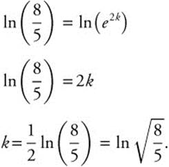
Step 3. Substitute 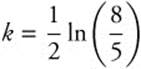 into one of the equations.
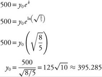
Thus, there are 395 bacteria present initially.
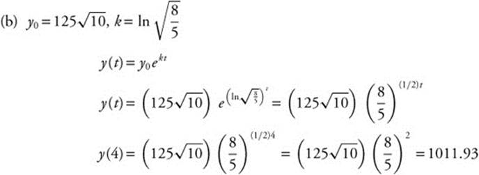
Thus there are approximately 1011 bacteria present after 4 days.
• Get a good night’s sleep the night before. Have a light breakfast before the exam.
Example 2—Radioactive Decay
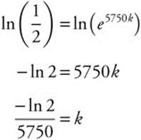
Carbon-14 has a half-life of 5750 years. If initially there are 60 grams of carbon-14, how many grams are left after 3000 years?
Step 1. y(t) = y0ekt = 60ekt
Since half-life is 5750 years, ![]() .
.
Step 2. y(t) = y0ekt
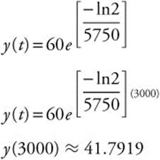
Thus, there will be approximately 41.792 grams of carbon-14 after 3000 years.
Separable Differential Equations
General Procedure

1. Separate the variables: g(y)dy = f(x)dx.
2. Integrate both sides: ![]() g(y)dy =
g(y)dy = ![]() f(x)dx.
f(x)dx.
3. Solve for y to get a general solution.
4. Substitute given conditions to get a particular solution.
5. Verify your result by differentiating.
Example 1
Given ![]() and
and ![]() , solve the differential equation.
, solve the differential equation.
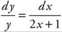
Step 1. Separate the variables: 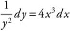 .
.
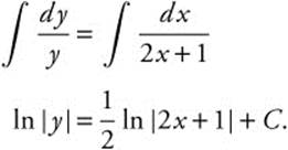
Step 2. Integrate both sides: 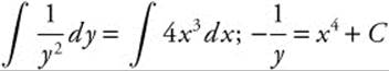 .
.
Step 3. General solution: ![]() .
.
Step 4. Particular solution: ![]() .
.
Step 5. Verify result by differentiating.
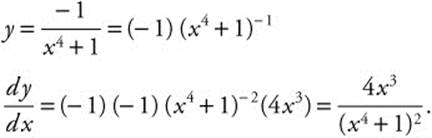
Note: ![]() implies
implies ![]() .
.
Thus, 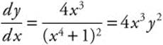 .
.
• To get your AP grade, you can call (888) 308-0013 in July. There is a charge of about $8.
Example 2
Find a solution of the differentiation equation ![]() ; y(0) = − 1.
; y(0) = − 1.
Step 1. Separate variables: dy = x sin(x2)dx.
Step 2. Integrate both sides: 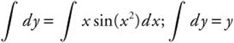 .
.
Let u = x2; du = 2x dx or ![]() .
.
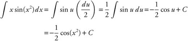
Thus, ![]() .
.
Step 3. Substitute given condition:
![]()
Thus, ![]() .
.
Step 4. Verify result by differentiating:
![]() .
.
Example 3
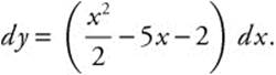
If ![]() and at x = 0, y′ = − 1, and y = 3, find a solution of the differential equation.
and at x = 0, y′ = − 1, and y = 3, find a solution of the differential equation.
Step 1. Rewrite ![]() as
as ![]() ;
; ![]() .
.
Step 2. Separate variables: dy′ = (2x + 1)dx.
Step 3. Integrate both sides: 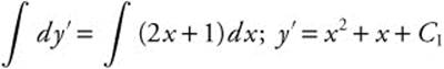 .
.
Step 4. Substitute given condition: At x = 0, y′ = − 1; − 1 = 0 + 0 + C1 ⇒ C1 = − 1. Thus, y′ = x2 + x − 1.
Step 5. Rewrite: ![]() .
.
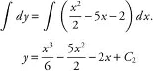
Step 6. Separate variables: dy = (x2 + x − 1)dx.
Step 7. Integrate both sides: 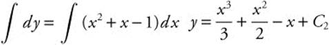 .
.
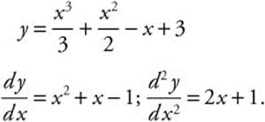
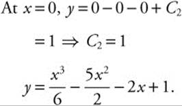
Step 8. Substitute given condition: At x = 0, y = 3; 3 = 0 + 0 − 0 + C2 ⇒ C2 = 3.
Therefore, ![]() .
.
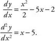
Step 9. Verify result by differentiating:
Example 4
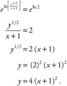
Find the general solution of the differential equation ![]() .
.
Step 1. Separate variables:
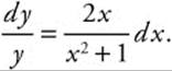
Step 2. Integrate both sides: 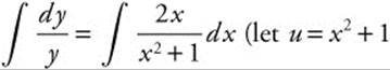 ; du = 2x dx) ln|y| = ln(x2 + 1) + C1.
Step 3. General Solution: solve for y.
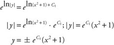
The general solution is y = C(x2 + 1).
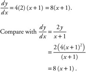
Step 4. Verify result by differentiating:
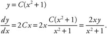
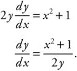
Example 5
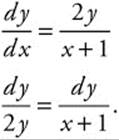
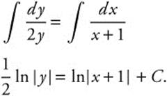
Write an equation for the curve that passes through the point (3, 4) and has a slope at any point (x, y) as 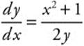 .
.
Step 1. Separate variables: 2y dy = (x2 + 1)dx.
Step 2. Integrate both sides: 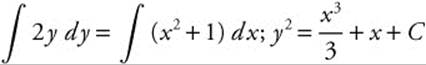 .
.
Step 3. Substitute given condition: ![]() .
.
Thus, ![]() .
.
Step 4. Verify the result by differentiating:
13.5 Slope Fields
Main Concepts: Slope Fields, Solution of Different Equations
A slope field (or a direction field) for first-order differential equations is a graphic representation of the slopes of a family of curves. It consists of a set of short line segments drawn on a pair of axes. These line segments are the tangents to a family of solution curves for the differential equation at various points. The tangents show the direction which the solution curves will follow. Slope fields are useful in sketching solution curves without having to solve a differential equation algebraically.
Example 1
If ![]() , draw a slope field for the given differential equation.
, draw a slope field for the given differential equation.
Step 1: Set up a table of values for ![]() for selected values of x.
for selected values of x.
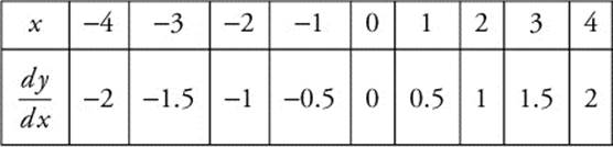
Note that since ![]() , the numerical value of
, the numerical value of ![]() is independent of the value of y. For example, at the points (1, − 1), (1, 0), (1, 1), (1, 2), (1, 3), and at all the points whose x-coordinates are 1, the numerical value of
is independent of the value of y. For example, at the points (1, − 1), (1, 0), (1, 1), (1, 2), (1, 3), and at all the points whose x-coordinates are 1, the numerical value of ![]() is 0.5 regardless of their y-coordinates. Similarly, for all the points, whose x-coordinates are 2 (e.g., (2, − 1), (2, 0), (2, 3), etc.),
is 0.5 regardless of their y-coordinates. Similarly, for all the points, whose x-coordinates are 2 (e.g., (2, − 1), (2, 0), (2, 3), etc.), ![]() . Also, remember that
. Also, remember that ![]() represents the slopes of the tangent lines to the curve at various points. You are now ready to draw these tangents.
represents the slopes of the tangent lines to the curve at various points. You are now ready to draw these tangents.
Step 2: Draw short line segments with the given slopes at the various points. The slope field for the differential equation ![]() is shown in Figure 13.5-1.
is shown in Figure 13.5-1.

Figure 13.5-1
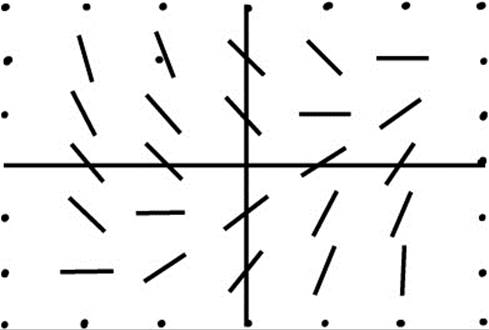
Example 2
Figure 13.5-2 shows a slope field for one of the differential equations given below. Identify the equation.
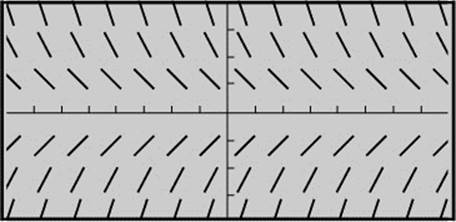
Figure 13.5-2
![]()
![]()
![]()
![]()
![]()
Solution:
If you look across horizontally at any row of tangents, you’ll notice that the tangents have the same slope. (Points on the same row have the same y-coordinate but different x-coordinates.) Therefore, the numerical value of ![]() (which represents the slope of the tangent) depends solely on the y-coordinate of a point and it is independent of the x-coordinate. Thus, only choice (c) and choice (d) satisfy this condition. Also notice that the tangents have a negative slope when y > 0 and have a positive slope when y < 0.
(which represents the slope of the tangent) depends solely on the y-coordinate of a point and it is independent of the x-coordinate. Thus, only choice (c) and choice (d) satisfy this condition. Also notice that the tangents have a negative slope when y > 0 and have a positive slope when y < 0.
Therefore, the correct choice is (c) ![]() .
.
Example 3
A slope field for a differential equation is shown in Figure 13.5-3. Draw a possible graph for the particular solution y = f(x) to the differential equation function, if (a) the initial condition is f (0) = − 2 and (b) the initial condition is f(0) = 0.
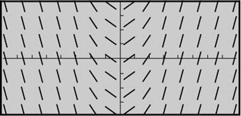
Figure 13.5-3
Solution:
Begin by locating the point (0, −2) as given in the initial condition. Follow the flow of the field and sketch the graph of the function. Repeat the same procedure with the point (0, 0). See the curves as shown in Figure 13.5-4.
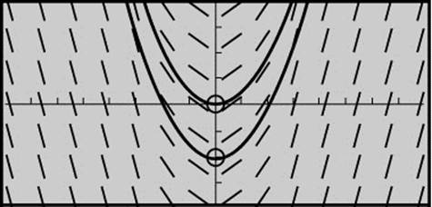
Figure 13.5-4
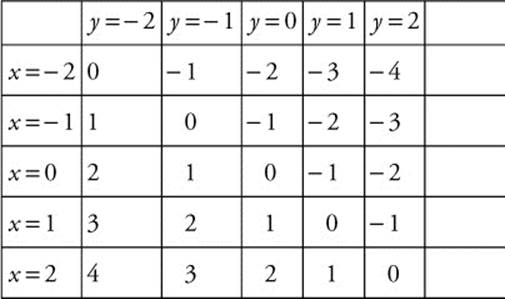
Example 4
Given the differential equation ![]() .
.
(a) Draw a slope field for the differential equation at the 15 points indicated on the provided set of axes in Figure 13.5-5.
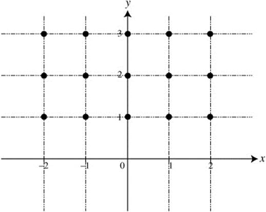
Figure 13.5-5
(b) Sketch a possible graph for the particular solution y = f(x) to the differential equation with the initial condition f(0) = 3.
(c) Find, algebraically, the particular solution y = f(x) to the differential equation with the initial condition f (0) = 3.
Solution:
(a) Set up a table of values for ![]() at the 15 given points.
at the 15 given points.
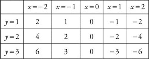
Then sketch the tangents at the various points as shown in Figure 13.5-6.
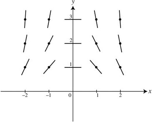
Figure 13.5-6
(b) Locate the point (0, 3) as indicated in the initial condition. Follow the flow of the field and sketch the curve as shown Figure 13.5-7.
(c)
Step 1: Rewrite ![]() as
as 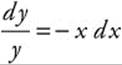 .
.
Step 2: Integrate both sides 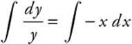 and obtain ln
 ![]() .
.
Step 3: Apply the exponential function to both sides and obtain ![]() .
.
Step 4: Simplify the equation and get 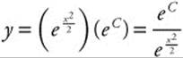 .
.
Let k = eC and you have  .
.
Step 5: Substitute initial condition (0, 3) and obtain k = 3. Thus, you have ![]() .
.
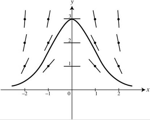
Figure 13.5-7

13.6 Logistic Differential Equations
Main Concepts: Logistic Growth
Often population may grow exponentially at first, but eventually slows as it nears a limit, called the carrying capacity. This patten is called logistic growth, and is represented by the differential equation 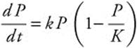 , in which P is the population, K is the carrying capacity, and k is the proportional constant. The differential equation is separable so
 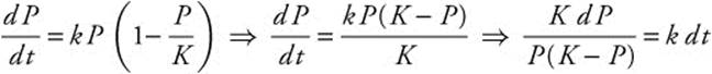 . This equation can be integrated using a partial fraction decomposition.
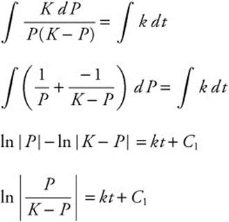
Exponention produces ![]() . Solving for P yields
. Solving for P yields ![]() . Dividing numerator and denominator by
. Dividing numerator and denominator by 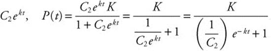 . At t = 0,
 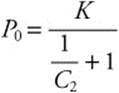 . Solving for C2 yields
 ![]() or
or ![]() . Let
. Let ![]() , and the solution of this logistic differential equation with initial condition
, and the solution of this logistic differential equation with initial condition ![]() where K is the carrying capacity and
where K is the carrying capacity and ![]() .
.
Example 1
The population of United Kingdom was 57.1 million in 2001 and 60.6 million in 2006. Find a logistic model for the growth of the population, assuming a carrying capacity of 100 million. Use the model to predict the population in 2020.
Step 1: Since the carrying capacity is K = 100, 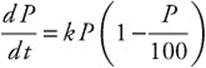 .
.
Step 2: The solution of the differential equation, if 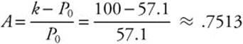 is
is ![]() or
or ![]() .
.
Step 3: Take 2006 as t = 5, P (5) = 60.6. Then ![]() . Solving gives
. Solving gives ![]() .
.
Step 4: Since the year 2020 corresponds to t = 19, Substitute and evaluate ![]() . The population of United Kingdom in 2020 is predicted to be approximately 69.742 million.
. The population of United Kingdom in 2020 is predicted to be approximately 69.742 million.
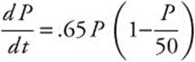
Example 2
The spread of an infectious disease can often be modeled by a logistic equation with the total exposed population as the carrying capacity. In a community of 2000 individuals, the first case of a new virus is diagnosed on March 31, and by April 10, there are 500 individuals infected. Write a differential equation that models the rate at which the virus spread through the community and determine when 98% of the population will have contracted the virus.
Step 1: The rate of spread is 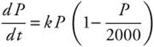 .
.
Step 2: The solution of the differential equation is ![]() , and with one person exposed,
, and with one person exposed, ![]() , or
, or ![]() .
.
Step 3: Taking April 10 as day 10, ![]() . Solving the equation gives k ≈.6502, so
. Solving the equation gives k ≈.6502, so ![]() .
.
Step 4: 98% of the population of 2000 is 1960 people. To determine the day when 1960 people are infected, solve ![]() . This gives t ≈ 17.6749, so the 98% infection rate should be reached by April 18.
. This gives t ≈ 17.6749, so the 98% infection rate should be reached by April 18.
13.7 Euler’s Method
Main Concept: Approximating Solutions of Differential Equations by Euler’s Method.
Approximating Solutions of Differential Equations by Euler’s Method
Euler’s Method provides a means of estimating the numerical solution of differential equations by a series of successive linear approximations. Represent the differential equation by y′ = f′(x, y) and the initial condition y0 = f(x0), and choose a small value, Δx, as the increment between estimates. Begin with the initial value y0, and evaluate ![]() . Continue with
. Continue with ![]() , and in general,
, and in general, ![]() .
.
Example 1
Given the initial value problem ![]() with y (0) = 1, approximate y (1), using five steps.
with y (0) = 1, approximate y (1), using five steps.
Step 1: The interval (0, 1) divided into five steps gives us Δt = 0.2.
Step 2: Create a table showing the iterations.
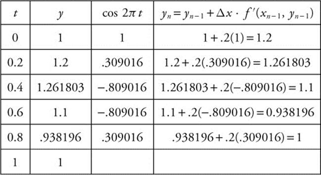
y (1) ≈ 1
Example 2
Use Euler’s method with a step size of Δx = 0.1 to compute y(1) if y(x) is the solution of the differential equation ![]() with initial condition y (0) = 3.
with initial condition y (0) = 3.
Step 1: For case of the evaluation, transform ![]() to
to ![]() .
.
Step 2: Create a table showing the iterations. A simple problem, stored in your calculator and modified with the new differential equation and initial condition, will allow you to generate the table quickly.
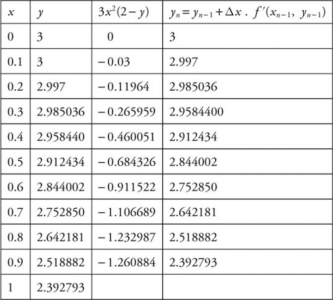
y (1) ≈ 2.393
Example 3
Use Euler’s Method to approximate P(4), given 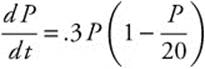 with initial condition P(0) = 4. Use an increment of Δt = 0.5.
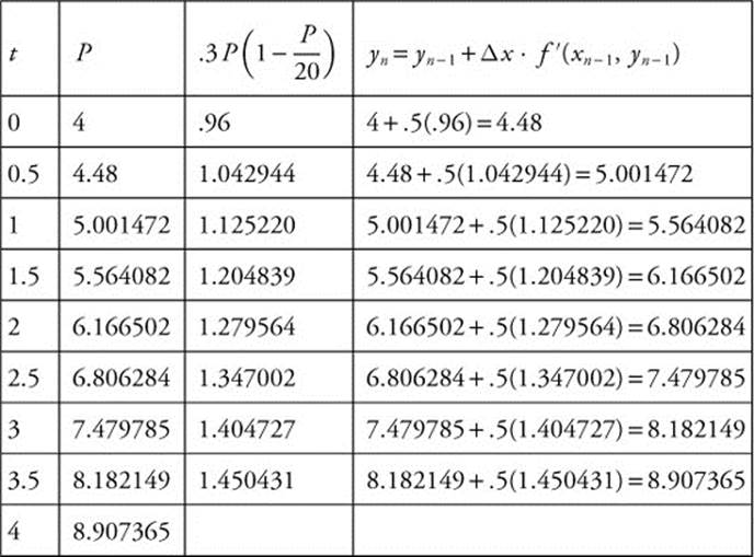
P (4) ≈ 8.907
13.8 Rapid Review
1. Find the average value of y = sin x on [0, π].
Answer:
 .
.
2. Find the total distance traveled by a particle during 0 ≤ t ≤ 3 whose velocity function is shown in Figure 13.8-1.
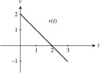
Figure 13.8-1
Answer:
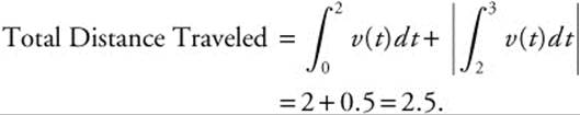 .
.
3. Oil is leaking from a tank at the rate of f(t) = 5e−0.1t gallons/hour, where t is measured in hours. Write an integral to find the total number of gallons of oil that will have leaked from the tank after 10 hours. Do not evaluate the integral.
Answer: Total number of gallons leaked 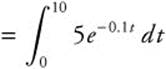 .
.
4. How much money should Mary invest at 7.5% interest a year compounded continuously, so that she will have $100,000 after 20 years.
Answer: y(t) = y0ekt, k = 0.075, and t = 20. y (20) = 100,000 = y0e(0.075)(20). Thus, using a calculator, you obtain y0 ≈ 22313, or $22,313.
5. Given  and y(1) = 0, solve the differential equation.
Answer: ![]()
Thus, ![]() or y2 = x2 − 1.
or y2 = x2 − 1.
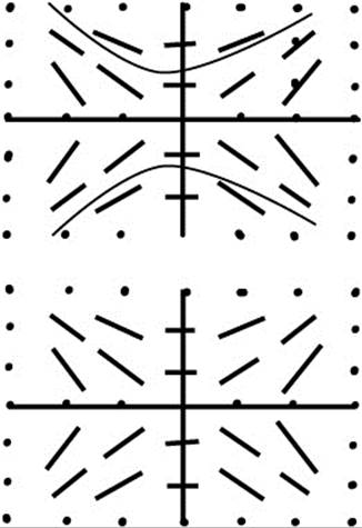
6. Identify the differential equation for the slope field shown.
Answer: The slope field suggests a hyperbola of the form y2 − x2 = k, so ![]() and
and  .
.
7. Find the solution of the initial value problem 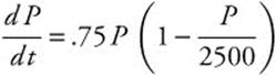 with P0 = 10.
8. Use Euler’s method with a step size of Δx = 0.5 to compute y (2), if y (x) is the solution of the differential equation ![]() with initial condition y (0) = 1.
with initial condition y (0) = 1.
Answer: y (0) = 1; y (0.5) = 1 + 0.5(1 + 0.1) = 1.5; y (1) = 1.5 + 0.5 [1.5 + (0.5)(1.5)] = 1.5 + 0.5[2.25] = 2.625 y (1.5) = 2.625 + 0.5 [2.625 + (1)(2.625)] = 2.625 + 2.625 = 5.25 y (2) = 5.25 + 0.5 [5.25 + (1.5)(5.25)] = 5.25 + 0.5[13.125] = 11.8125
13.9 Practice Problems
Part A—The use of a calculator is not allowed.
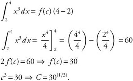
1. Find the value of c as stated in the Mean Value Theorem for Integrals for f(x) = x3 on [2, 4].
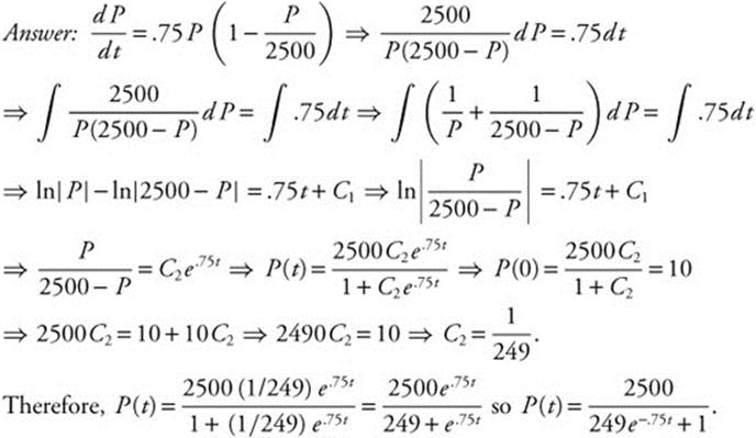
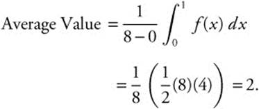
2. The graph of f is shown in Figure 13.9-1. Find the average value of f on [0, 8].
Figure 13.9-1
3. The position function of a particle moving on a coordinate line is given as s (t) = t2 − 6t − 7, 0 ≤ t ≤ 10. Find the displacement and total distance traveled by the particle from 1 ≤ t ≤ 4.
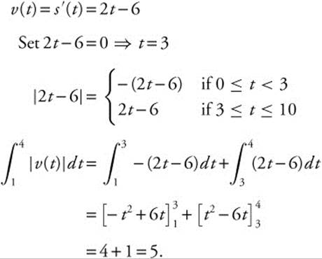
4. The velocity function of a moving particle on a coordinate line is v(t) = 2t + 1 for 0 ≤ t ≤ 8. At t = 1, its position is − 4. Find the position of the particle at t = 5.
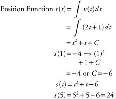
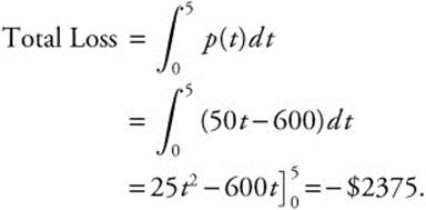
5. The rate of depreciation for a new piece of equipment at a factory is given as p(t) = 50t − 600 for 0 ≤ t ≤ 10, where t is measured in years. Find the total loss of value of the equipment over the first 5 years.
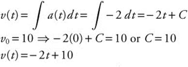
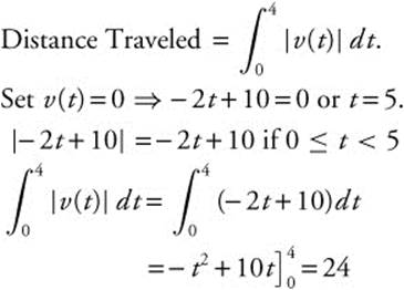
6. If the acceleration of a moving particle on a coordinate line is a(t) = − 2 for 0 ≤ t ≤ 4, and the initial velocity v0 = 10, find the total distance traveled by the particle during 0 ≤ t ≤ 4.
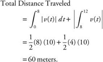
7. The graph of the velocity function of a moving particle is shown in Figure 13.9-2. What is the total distance traveled by the particle during 0 ≤ t ≤ 12?
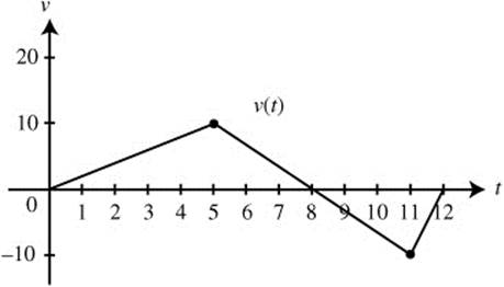
Figure 13.9-2
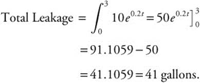
8. If oil is leaking from a tanker at the rate of f(t) = 10e0.2t gallons per hour where t is measured in hours, how many gallons of oil will have leaked from the tanker after the first 3 hours?
9. The change of temperature of a cup of coffee measured in degrees Fahrenheit in a certain room is represented by the function ![]() for 0 ≤ t ≤ 5, where t is measured in minutes. If the temperature of the coffee is initially 92°F, find its temperature after the first 5 minutes.
for 0 ≤ t ≤ 5, where t is measured in minutes. If the temperature of the coffee is initially 92°F, find its temperature after the first 5 minutes.
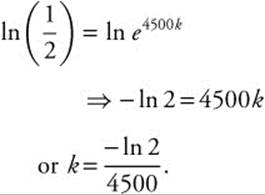
10. If the half-life of a radioactive element is 4500 years, and initially there are 100 grams of this element, approximately how many grams are left after 5000 years?
11. Find a solution of the differential equation:
![]() ; y(0) = π
; y(0) = π
12. If ![]() and at x = 0, y′ = − 2 and y = 1, find a solution of the differential equation.
and at x = 0, y′ = − 2 and y = 1, find a solution of the differential equation.
Part B—Calculators are allowed.
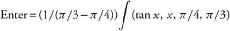
13. Find the average value of y = tan x from ![]() to
to ![]() .
.
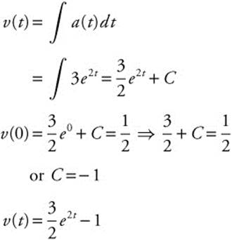
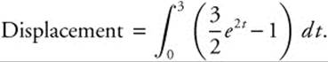
14. The acceleration function of a moving particle on a straight line is given by a(t) = 3e2t, where t is measured in seconds, and the initial velocity is ![]() . Find the displacement and total distance traveled by the particle in the first 3 seconds.
. Find the displacement and total distance traveled by the particle in the first 3 seconds.
15. The sales of an item in a company follow an exponential growth/decay model, where t is measured in months. If the sales drop from 5000 units in the first month to 4000 units in the third month, how many units should the company expect to sell during the seventh month?
16. Find an equation of the curve that has a slope of ![]() at the point (x, y) and passes through the point (0, 4).
at the point (x, y) and passes through the point (0, 4).
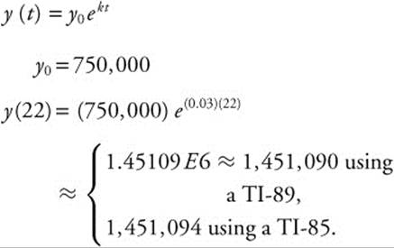
17. The population in a city was approximately 750,000 in 1980, and grew at a rate of 3% per year. If the population growth followed an exponential growth model, find the city’s population in the year 2002.
18. Find a solution of the differential equation 4ey = y′ − 3xey and y (0) = 0.
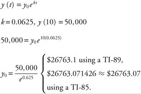
19. How much money should a person invest at 6.25% interest compounded continuously so that the person will have $50,000 after 10 years?
20. The velocity function of a moving particle is given as v(t) = 2 − 6e−t, t ≥ 0 and t is measured in seconds. Find the total distance traveled by the particle during the first 10 seconds.
21. Draw a slope field for the differential equation ![]() .
.
22. A rumor spreads through an office of fifty people at a model by 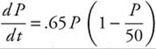 . On day zero, one person knows the rumor. Find the model for the population at time t, and use it to predict when more than half the people in the office will have heard the rumor.
23. A college dormitory that houses 200 students experiences an outbreak of influenza. The illness is recognized when two students are diagnosed on the same day. The residents are quarantined to restrict the infection to this one building. On the fifth day of the outbreak, 12 students are ill. Use a logistic model to describe the course of infection and predict the number of infected students on day 10.
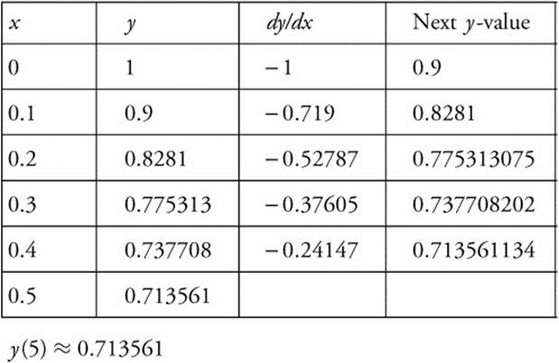
24. Use Euler’s Method with a step size of Δx = 0.1 to compute y (.5) if y (x) is the solution of the differential equation ![]() with the condition y (0) = 1.
with the condition y (0) = 1.
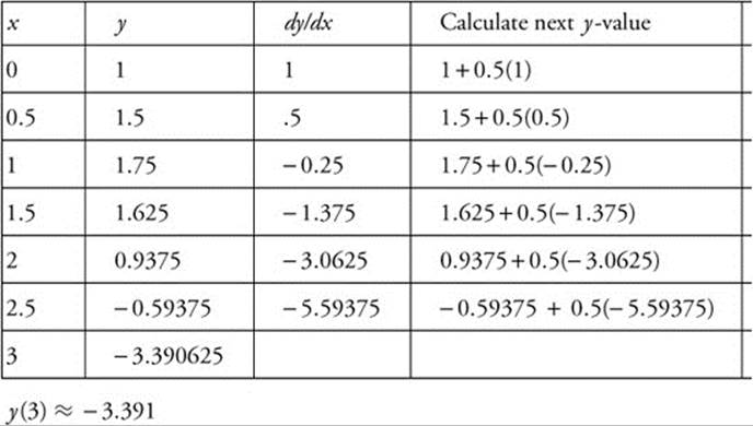
25. Use Euler’s Method with a step size of Δx = 0.5 to compute y (3) if y (x) is the solution of the differential equation ![]() with initial condition y(0) = 1.
with initial condition y(0) = 1.
13.10 Cumulative Review Problems
(Calculator) indicates that calculators are permitted.
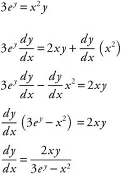
26. If 3ey = x2y, find ![]() .
.
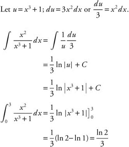
27. Evaluate 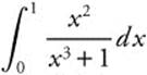 .
.
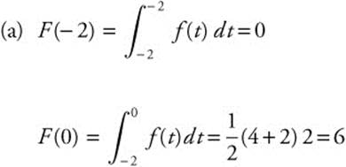
28. The graph of a continuous function f which consists of three line segments on [−2, 4] is shown in Figure 13.10-1. If 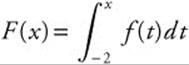 for − 2 ≤ x ≤ 4,
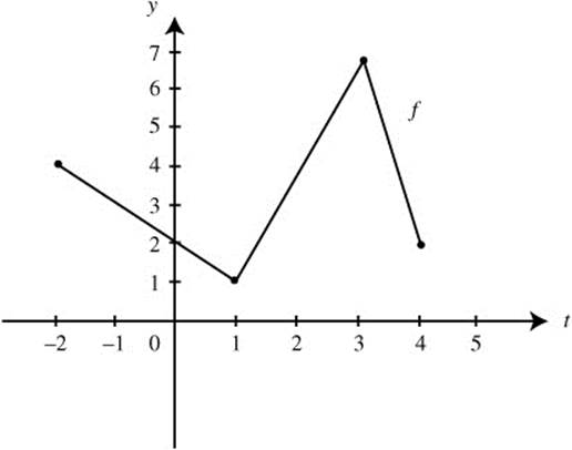
Figure 13.10-1
(a) Find F(− 2) and f(0).
(b) Find F′(0) and F′(2).
(c) Find the value of x such that F has a maximum on [− 2, 4].
(d) On which interval is the graph of F concave upward?
29. (Calculator) The slope of a function y = f(x) at any point (x, y) is ![]() and f(0) = 2.
and f(0) = 2.
(a) Write an equation of the line tangent to the graph of f at x = 0.
(b) Use the tangent in part (a) to find the approximate value of f(0.1).
(c) Find a solution y = f(x) for the differential equation.
(d) Using the result in part (c), find f(0.1).
30. (Calculator) Let R be the region in the first quadrant bounded by f(x) = ex − 1 and g(x) = 3 sin x.
(a) Find the area of region R.
(b) Find the volume of the solid obtained by revolving R about the x-axis.
(c) Find the volume of the solid having R as its base and semicircular cross sections perpendicular to the x-axis.
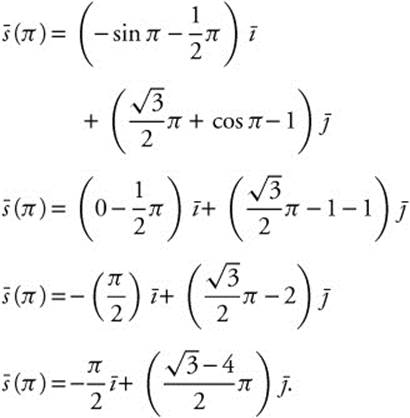
31. An object traveling on a path defined by ⟨x(θ), y(θ)⟩ has an acceleration vector of ⟨sinθ, − cos θ⟩. If the velocity of the object at time ![]() is ⟨− 1, 0⟩ and the initial position of the object is the origin, find the position when θ = π.
is ⟨− 1, 0⟩ and the initial position of the object is the origin, find the position when θ = π.
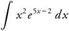
32. 
33. A projectile follows a path defined by x = t − 2, y = sin2 t on the interval 0 ≤ t ≤ π. Find the point at which the object reaches its maximum y-value.
13.11 Solutions to Practice Problems
Part A—The use of a calculator is not allowed.
1.
2.
3. Displacement = s(4) − s(1) = − 15 − (− 12) = − 3. Distance Traveled 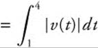 .
.
4.
5.
6.
7.
8.
9.
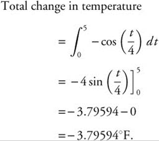
Thus the temperature of coffee after 5 minutes is (92 − 3.79594) ≈ 88.204°F.
10.
![]()
Half-life = 4500 ![]() . Take ln of both sides:
. Take ln of both sides:
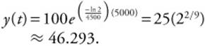
There are approximately 46.29 grams left.
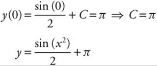
11. Step 1. Separate variables: dy = x cos(x2) dx.
Step 2. Integrate both sides:
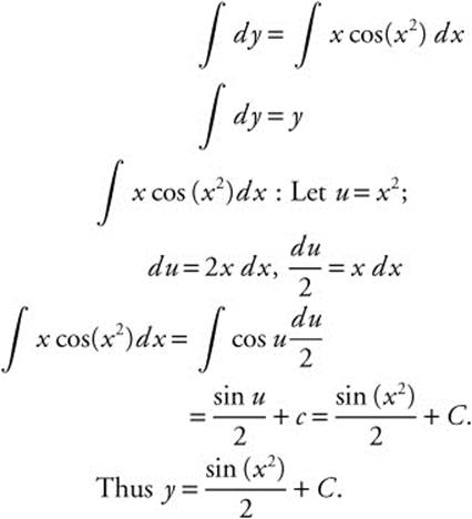
Step 3. Substitute given values.
Step 4. Verify result by differentiating:
![]()
12. Step 1.
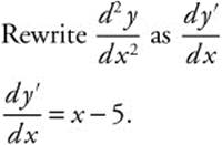 .
.
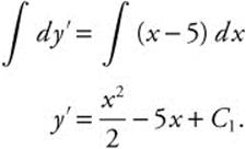
Step 2. Separate variables: dy′ = (x − 5)dx.
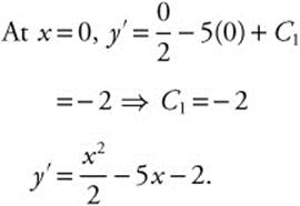
Step 3. Integrate both sides:
Step 4. Substitute given values:
Step 5. Rewrite: ![]()
Step 6. Separate variables:
Step 7. Integrate both sides:
Step 8. Substitute given values:
Step 9. Verify result by differentiating:
Part B—Calculators are allowed.
13. Average 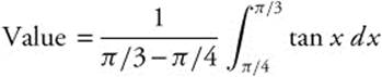 .
.
 and
and![]()
14.
Enter 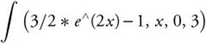 and obtain 298.822.
Distance 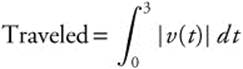 .
.
![]() for t ≥ 0,
for t ≥ 0, 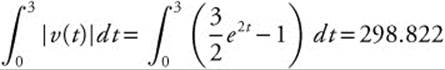
15. Step 1.
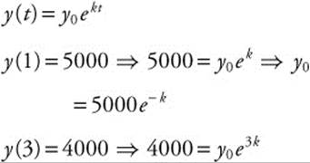
Substituting:
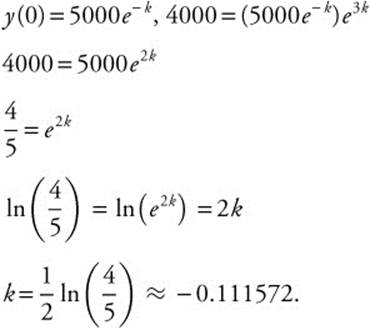
Step 2. 5000 = y0e−0.111572
y(0) = (5000)/e−0.111572 ≈ 5590.17
y(t) = (5590.17) e−0.111572
Step 3. y(7) = (5590.17)e−0.111572(7)
≈ = 2560
Thus, sales for the 7th month are approximately 2560 units.
16. Step 1. Separate variables:
Step 2. Integrate both sides:
Step 3. Substitute given value (0, 4):
Step 4. Verify result by differentiating:
17.
18. Step 1. Separate variables:
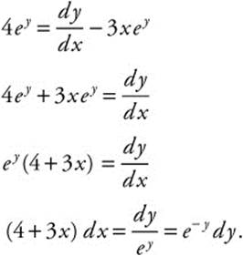
Step 2. Integrate both sides:
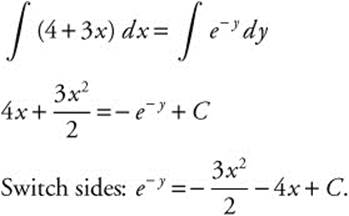
Step 3. Substitute given value: y (0) = 0
⇒ e0 = 0 − 0 + c ⇒ c = 1.
Step 4. Take ln of both sides:
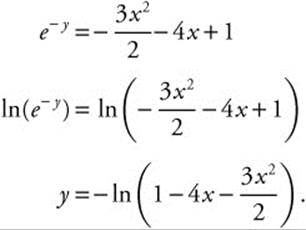
Step 5. Verify result by differentiating: Enter d(− ln(1 − 4x − 3 (x − ^2)/2), x) and obtain ![]() , which is equivalent to ey(4 + 3x).
, which is equivalent to ey(4 + 3x).
19.
20. Set v(t) = 2 − 6e−t = 0. Using the [Zero] function on your calculator, compute t = 1.09861.
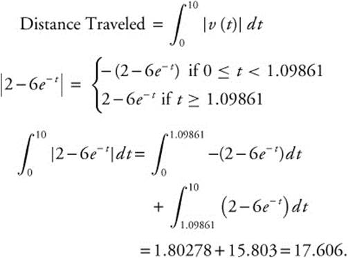
Alternatively, use the [nInt] function on the calculator.
Enter nInt(abs(2 − 6e^(− x)), x, 0, 10) and obtain the same result.
21. Build a table of value for ![]() .
.
Draw short lines at each intersection with slopes equal to the value of ![]() at that point.
at that point.
22.  can be separated and integrated by partial fractions.
 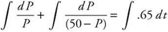 produces ln |P| + ln |50 − P| = .65t + C1 and
 ![]() , so
, so 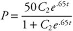 . Since one person knows the rumor on day zero,
 ![]() and
and ![]() . The model for the population becomes
. The model for the population becomes 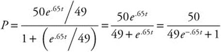 . Half the population of the office would be 25 people, so solve for t in
 ![]() . Since t ≈ 5.987, half of the office will have heard the rumor by the sixth day.
. Since t ≈ 5.987, half of the office will have heard the rumor by the sixth day.
23. The logistic model becomes 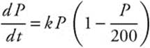 since the carrying capacity is 200. Separate the variables
 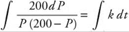 and integrate by partial fractions
 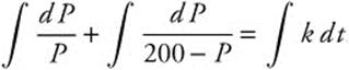 . You find ln
 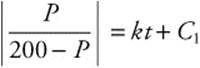 . Exponentiate to get
 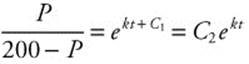 . Solving for P produces
 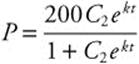 . On day zero, two students are infected, so
 ![]() and
and ![]() . On day five, 12 students are infected, so
. On day five, 12 students are infected, so 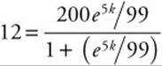 and k ≈ .369.
Therefore, 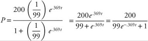 . On day 10,
 ![]() , so we would predict that approximately 58 students would be infected on the tenth day.
, so we would predict that approximately 58 students would be infected on the tenth day.
24. Apply ![]() with Δx = 0.1. (See table below.)
with Δx = 0.1. (See table below.)
25. Apply ![]() with Δx = 0.5. (See table below.)
with Δx = 0.5. (See table below.)
Solution to Problem 24.
Solution to Problem 25.
13.12 Solutions to Cumulative Review Problems
26.
27.
28.
(b) F′(x) = f(x); F′(0) = 2 and F′(2) = 4.
(c) Since f > 0 on [−2, 4], F has a maximum value at x = 4.
(d) The function f is increasing on (1, 3) which implies that f′ > 0 on (1, 3). Thus, F is concave upward on (1, 3). (Note: f′ is equivalent to the 2nd derivative of F.)
29.
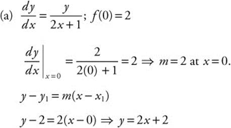
The equation of the tangent to f at x = 0 is y = 2x + 2.
(b) f(0.1) = 2(0.1) + 2 = 2.2
(c) Solve the differential equation: ![]() .
.
Step 1. Separate variables:
Step 2. Integrate both sides:
Step 3. Substitute given values (0, 2):
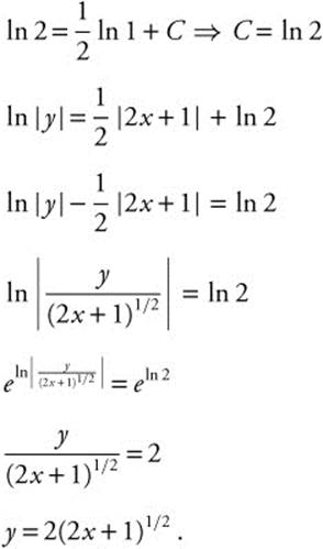
Step 4. Verify result by differentiating
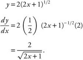
Compare this with:
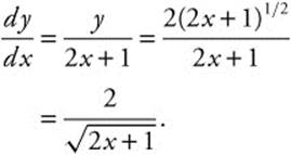
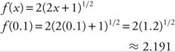
Thus, the function is y = f(x) = 2(2x + 1)1/2.
(d)
30. See Figure 13.12-1.
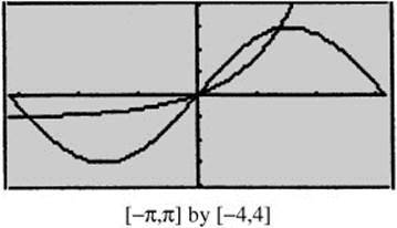
Figure 13.12-1
(a) Intersection points: Using the [Intersection] function on the calculator, you have x = 0 and x = 1.37131.
Area of 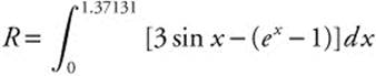 .
.
Enter 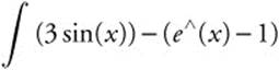 , x, 0, 1.37131 and obtain 0.836303. The area of region R is approximately 0.836.
(b) Using the Washer Method, volume of 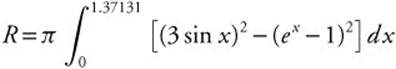 . Enter
 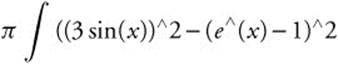 , x, 0, 1.37131) and obtain 2.54273π or 7.98824.
The volume of the solid is 7.988.
(c) Volume of Solid =  (Area of Cross Section)dx.
Area of Cross 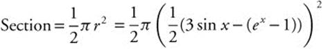 .
.
Enter 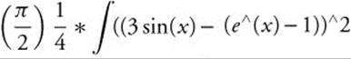 , x, 0, 1.37131) and obtain 0.077184 π or 0.24248.
The volume of the solid is approximately 0.077184 π or 0.242.
31. Integrate the acceleration vector to get the velocity vector:
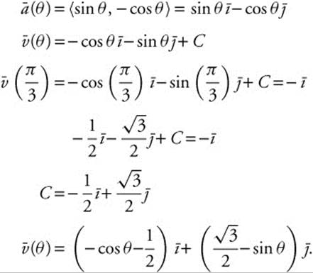
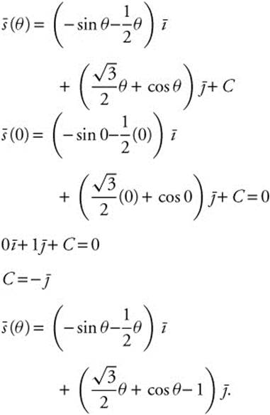
Integrate the velocity vector to get the position vector:
Substituting in θ = π:
32. Integrate 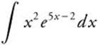 by parts. Let u = x2, du = 2x dx, dv = e5x − 2 dx, and
 ![]() . Then,
. Then, 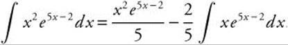 . The remaining integral can be evaluated by parts, using u = x, du = dx, dv = e5x − 2 dx, and
 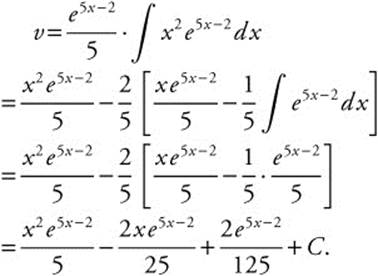 .
.
33. The path is defined by x = t − 2, y = sin2 t. Since ![]() and
and ![]() ,
, ![]() . This is the slope of a tangent line to the curve, and when the slope is zero, the curve will reach either a maximum or a minimum. The slope 2 sin t cos t = 0 when sin t = 0 or when cos t = 0. The first equation gives us t = 0 or t = π and the second,
. This is the slope of a tangent line to the curve, and when the slope is zero, the curve will reach either a maximum or a minimum. The slope 2 sin t cos t = 0 when sin t = 0 or when cos t = 0. The first equation gives us t = 0 or t = π and the second, ![]() . The second derivative,
. The second derivative, 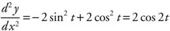 . Evaluating at each of the possible values of t, we find 2 cos
 ![]() ,
, ![]() , and
, and ![]() . The maximum value will occur when the second derivative is negative, so the maximum y-value is achieved when
. The maximum value will occur when the second derivative is negative, so the maximum y-value is achieved when ![]() ,
, ![]() , and
, and ![]() .
.