5 Steps to a 5 AP Calculus AB & BC, 2012-2013 Edition (2011)
STEP 4. Review the Knowledge You Need to Score High
Chapter 7. Graphs of Functions and Derivatives
IN THIS CHAPTER
Summary: Many questions on the AP Calculus exams involve working with graphs of a function and its derivatives. In this chapter, you will learn how to use derivatives both algebraically and graphically to determine the behavior of a function. Applications of Rolle’s Theorem, the Mean Value Theorem, and the Extreme Value Theorem are shown. You will also learn to sketch the graphs of parametric and polar equations.

Key Ideas
![]() Rolle’s Theorem, Mean Value Theorem, and Extreme Value Theorem
Rolle’s Theorem, Mean Value Theorem, and Extreme Value Theorem
![]() Test for Increasing and Decreasing Functions
Test for Increasing and Decreasing Functions
![]() First and Second Derivative Tests for Relative Extrema
First and Second Derivative Tests for Relative Extrema
![]() Test for Concavity and Point of Inflection
Test for Concavity and Point of Inflection
![]() Curve Sketching
Curve Sketching
![]() Graphs of Derivatives
Graphs of Derivatives
![]() Parametric and Polar Equations
Parametric and Polar Equations
![]() Vectors
Vectors
7.1 Rolle’s Theorem, Mean Value Theorem, and Extreme Value Theorem
Main Concepts:
Rolle’s Theorem, Mean Value Theorem, Extreme Value Theorem

• Set your calculator to Radians and change it to Degrees if/when you need to. Do not forget to change it back to Radians after you have finished using it in Degrees.
Rolle’s Theorem
If f is a function that satisfies the following three conditions:
1. f is continuous on a closed interval [a, b]
2. f is differentiable on the open interval (a, b)
3. f(a) = f(b) = 0
then there exists a number c in (a, b) such that f’(c) = 0. (See Figure 7.1-1.)
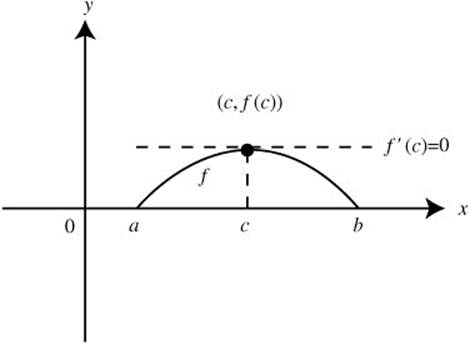
Figure 7.1-1
Note that if you change condition 3 from f(a) = f(b) = 0 to f(a) = f(b), the conclusion of Rolle’s Theorem is still valid.
Mean Value Theorem
If f is a function that satisfies the following conditions:
1. f is continuous on a closed interval [a, b]
2. f is differentiable on the open interval (a, b)
then there exists a number c in (a, b) such that ![]() . (See Figure 7.1-2.)
. (See Figure 7.1-2.)
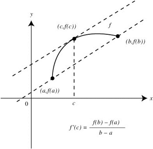
Figure 7.1-2
Example 1
If f(x) = x2 + 4x − 5, show that the hypotheses of Rolle’s Theorem are satisfied on the interval [− 4, 0] and find all values of c that satisfy the conclusion of the theorem. Check the three conditions in the hypothesis of Rolle’s Theorem:
(1) f(x) = x2 + 4x − 5 is continuous everywhere since it is polynomial.
(2) The derivative f′(x) = 2x + 4 is defined for all numbers and thus is differentiable on (− 4, 0).
(3) f(0) = f (− 4) = − 5. Therefore, there exists a c in (− 4, 0) such that f′(c) = 0. To find c, set f′(x) = 0. Thus, 2x + 4 = 0 ⇒ x = − 2, i.e., f′(− 2) = 0. (See Figure 7.1-3.)
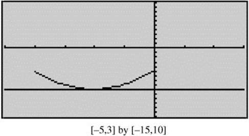
Figure 7.1-3
Example 2
Let ![]() . Using Rolle’s Theorem, show that there exists a number c in the domain of f such that f′(c) = 0. Find all values of c.
. Using Rolle’s Theorem, show that there exists a number c in the domain of f such that f′(c) = 0. Find all values of c.
Note f(x) is a polynomial and thus f(x) is continuous and differentiable everywhere.
Enter ![]() . The zeros of y1 are approximately − 2.3, 0.9, and 2.9 i.e., f(− 2.3) = f(0.9) = f(2.9) = 0. Therefore, there exists at least one c in the interval (− 2.3, 0.9) and at least one c in the interval (0.9, 2.9) such that f′(c) = 0. Use d[Differentiate] to find f′(x): f′(x) = x2 − x − 2. Set f′(x) = 0 ⇒ x2 − x − 2 = 0 or (x − 2)(x + 1) = 0.
. The zeros of y1 are approximately − 2.3, 0.9, and 2.9 i.e., f(− 2.3) = f(0.9) = f(2.9) = 0. Therefore, there exists at least one c in the interval (− 2.3, 0.9) and at least one c in the interval (0.9, 2.9) such that f′(c) = 0. Use d[Differentiate] to find f′(x): f′(x) = x2 − x − 2. Set f′(x) = 0 ⇒ x2 − x − 2 = 0 or (x − 2)(x + 1) = 0.
Thus, x = 2 or x = − 1, which implies f′(2) = 0 and f′(− 1) = 0. Therefore, the values of c are − 1 and 2. (See Figure 7.1-4.)
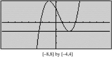
Figure 7.1-4
Example 3
The points P(1, 1) and Q(3, 27) are on the curve f(x) = x3. Using the Mean Value Theorem, find c in the interval (1, 3) such that f′(c) is equal to the slope of the secant ![]() .
.
The slope of secant ![]() is
is ![]() . Since f(x) is defined for all real numbers, f(x) is continuous on [1, 3]. Also f′(x) = 3x2 is defined for all real numbers. Thus, f(x) is differentiable on (1, 3). Therefore, there exists a number c in (1, 3) such that f′(c) = 13. Set f′(c) = 13 ⇒ 3(c)2 = 13 or
. Since f(x) is defined for all real numbers, f(x) is continuous on [1, 3]. Also f′(x) = 3x2 is defined for all real numbers. Thus, f(x) is differentiable on (1, 3). Therefore, there exists a number c in (1, 3) such that f′(c) = 13. Set f′(c) = 13 ⇒ 3(c)2 = 13 or 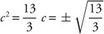 . Since only
 ![]() is in the interval (1, 3),
is in the interval (1, 3),  . (See Figure 7.1-5.)
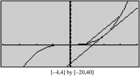
Figure 7.1-5
Example 4
Let f be the function f(x) = (x − 1)2/3. Determine if the hypotheses of the Mean Value Theorem are satisfied on the interval [0, 2], and if so, find all values of c that satisfy the conclusion of the theorem.
Enter y1 = (x − 1)2/3. The graph y1 shows that there is a cusp at x = 1. Thus, f(x) is not differentiable on (0, 2) which implies there may or may not exist a c in (0, 2) such that 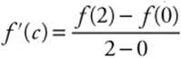 . The derivative
 ![]() and
and ![]() . Set
. Set ![]() . Note that f is not differentiable (a + x = 1). Therefore, c does not exist. (See Figure 7.1-6.)
. Note that f is not differentiable (a + x = 1). Therefore, c does not exist. (See Figure 7.1-6.)
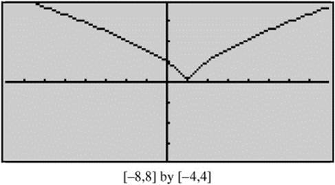
Figure 7.1-6
• The formula for finding the area of an equilateral triangle is ![]()
where s is the length of a side. You might need this to find the volume of a solid whose cross sections are equilateral triangles.
Extreme Value Theorem
If f is a continuous function on a closed interval [a, b], then f has both a maximum and a minimum value on the interval.
Example 1
If f(x) = x3 + 3x2 − 1, find the maximum and minimum values of f on [− 2, 2]. Since f(x) is a polynomial, it is a continuous function everywhere. Enter y1 = x3 + 3x2 − 1. The graph of y1 indicates that f has a minimum of − 1 at x = 0 and a maximum value of 19 at x = 2. (See Figure 7.1-7.)
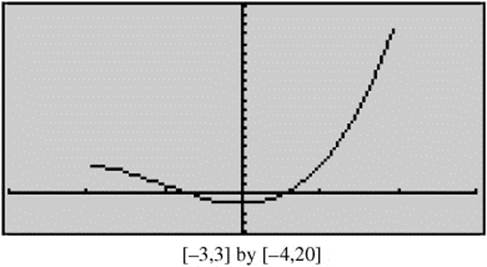
Figure 7.1-7
Example 2
If ![]() , find any maximum and minimum values of f on [0, 3]. Since f(x) is a rational function, it is continuous everywhere except at values where the denominator is 0. In this case, at x = 0, f(x) is undefined. Since f(x) is not continuous on [0, 3], the Extreme Value Theorem may not be applicable. Enter
, find any maximum and minimum values of f on [0, 3]. Since f(x) is a rational function, it is continuous everywhere except at values where the denominator is 0. In this case, at x = 0, f(x) is undefined. Since f(x) is not continuous on [0, 3], the Extreme Value Theorem may not be applicable. Enter ![]() . The graph of y1 shows that as x → 0+, f(x) increases without bound (i.e., f(x) goes to infinity). Thus, f has no maximum value. The minimum value occurs at the endpoint x = 3 and the minimum value is
. The graph of y1 shows that as x → 0+, f(x) increases without bound (i.e., f(x) goes to infinity). Thus, f has no maximum value. The minimum value occurs at the endpoint x = 3 and the minimum value is ![]() . (See Figure 7.1-8.)
. (See Figure 7.1-8.)
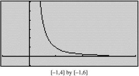
Figure 7.1-8
7.2 Determining the Behavior of Functions
Main Concepts:
Test for Increasing and Decreasing Functions, First Derivative Test and Second Derivative Test for Relative Extrema, Test for Concavity and Points of Inflection
Test for Increasing and Decreasing Functions
Let f be a continuous function on the closed interval [a, b] and differentiable on the open interval (a, b).
1. If f′(x) > 0 on (a, b), then f is increasing on [a, b].
2. If f′(x) < 0 on (a, b), then f is decreasing on [a, b].
3. If f′(x) = 0 on (a, b), then f is constant on [a, b].
Definition: Let f be a function defined at a number c. Then c is a critical number of f if either f′(c) = 0 or f′(c) does not exist. (See Figure 7.2-1.)
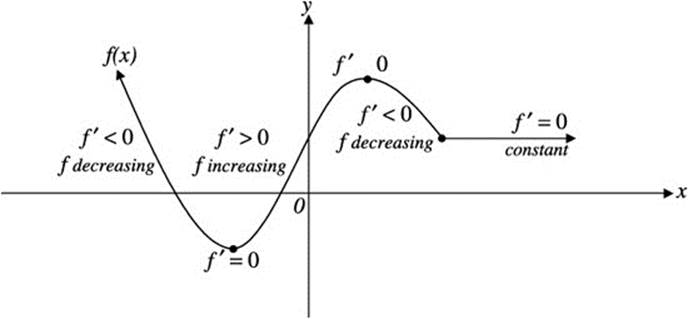
Figure 7.2-1
Example 1
Find the critical numbers of f(x) = 4x3 + 2x2.
To find the critical numbers of f(x), you have to determine where f′(x) = 0 and where f′(x) does not exist. Note f′(x) = 12x2 + 4x, and f′(x) is defined for all real numbers. Let f′(x) = 0 and thus 12x2 + 4x = 0, which implies 4x(3x + 1) = 0 ⇒ x = − 1/3 or x = 0. Therefore, the critical numbers of f are 0 and − 1/3. (See Figure 7.2-2.)
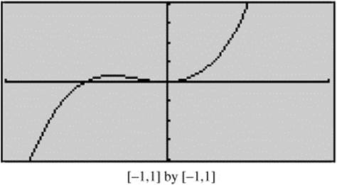
Figure 7.2-2
Example 2
Find the critical numbers of f(x) = (x − 3)2/5.
![]() . Note that f′(x) is undefined at x = 3 and that f′(x) ≠ 0. Therefore, 3 is the only critical number of f. (See Figure 7.2-3.)
. Note that f′(x) is undefined at x = 3 and that f′(x) ≠ 0. Therefore, 3 is the only critical number of f. (See Figure 7.2-3.)
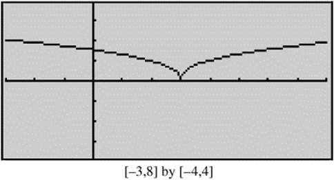
Figure 7.2-3
Example 3
The graph of f′ on (1, 6) is shown in Figure 7.2-4. Find the intervals on which f is increasing or decreasing.
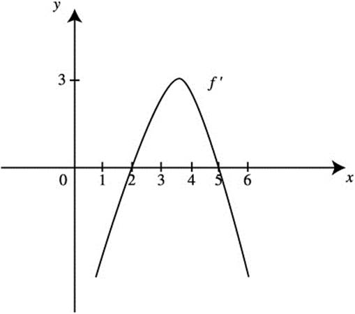
Figure 7.2-4
(See Figure 7.2-5.)
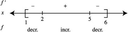
Figure 7.2-5
Thus, f is decreasing on [1, 2] and [5, 6] and increasing on [2, 5].
Example 4
Find the open intervals on which f(x) = (x2 − 9)2/3 is increasing or decreasing.
Step 1: Find the critical numbers of f.
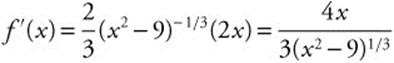
Set f′(x) = 0 ⇒ 4x = 0 or x = 0.
Since f′(x) is a rational function, f′(x) is undefined at values where the denominator is 0. Thus, set x2 − 9 = 0 ⇒ x = 3 or x = − 3. Therefore, the critical numbers are − 3, 0, and 3.
Step 2: Determine intervals.
![]()
Intervals are (− ∞, − 3), (− 3, 0), (0, 3), and (3, ∞).
Step 3: Set up a table.
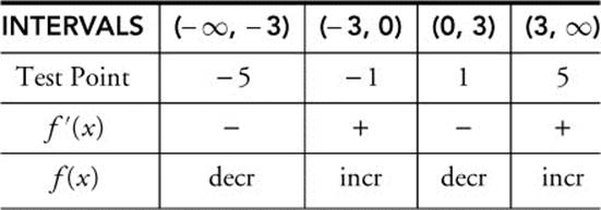
Step 4: Write a conclusion. Therefore, f(x) is increasing on [− 3, 0] and [3, ∞) and decreasing on (− ∞, − 3] and [0, 3]. (See Figure 7.2-6.)
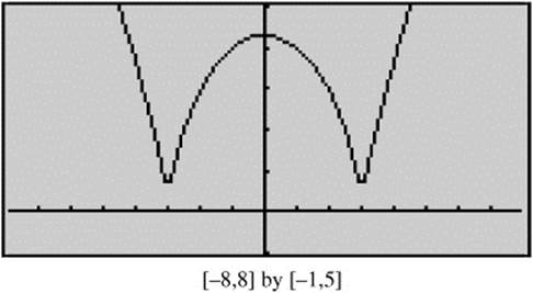
Figure 7.2-6
Example 5
The derivative of a function f is given as f′(x) = cos(x2). Using a calculator, find the values
of x on ![]() such that f is increasing. (See Figure 7.2-7.)
such that f is increasing. (See Figure 7.2-7.)
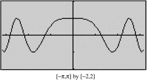
Figure 7.2-7
Using the [Zero] function of the calculator, you obtain x = 1.25331 is a zero of f′ on ![]() . Since f′(x) = cos(x2) is an even function, x = − 1.25331 is also a zero on
. Since f′(x) = cos(x2) is an even function, x = − 1.25331 is also a zero on ![]() . (See Figure 7.2-8.)
. (See Figure 7.2-8.)
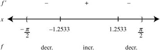
Figure 7.2-8
Thus, f is increasing on [− 1.2533, 1.2533].
• Bubble in the right grid. You have to be careful in filling in the bubbles especially when you skip a question.
First Derivative Test and Second Derivative Test for Relative Extrema
First Derivative Test for Relative Extrema
Let f be a continuous function and c be a critical number of f. (Figure 7.2-9.)
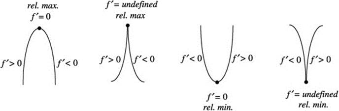
Figure 7.2-9
1. If f′(x) changes from positive to negative at x = c (f′ > 0 for x < c and f′ < 0 for x > c), then f has a relative maximum at c.
2. If f′(x) changes from negative to positive at x = c (f′ < 0 for x < c and f′ > 0 for x > c), then f has a relative minimum at c.
Second Derivative Test for Relative Extrema
Let f be a continuous function at a number c.
1. If f′(c) = 0 and f″(c) < 0, then f(c) is a relative maximum.
2. If f′(c) = 0 and f″(c) > 0, then f(c) is a relative minimum.
3. If f′(c) = 0 and f″(c) = 0, then the test is inconclusive. Use the First Derivative Test.
Example 1
The graph of f′, the derivative of a function f, is shown in Figure 7.2-10. Find the relative extrema of f.
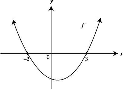
Figure 7.2-10
Solution: (See Figure 7.2-11.)
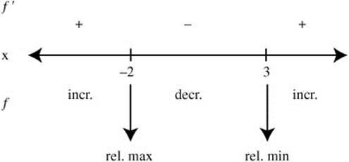
Figure 7.2-11
Thus, f has a relative maximum at x = − 2, and a relative minimum at x = 3.
Example 2
Find the relative extrema for the function ![]() .
.
Step 1: Find f′(x).
f′(x) = x2 − 2x − 3
Step 2: Find all critical numbers of f(x).
Note that f′(x) is defined for all real numbers. Set f′(x) = 0: x2 − 2x − 3 = 0 ⇒ (x − 3)(x + 1) = 0 ⇒ x = 3 or x = − 1.
Step 3: Find f″(x): f″(x) = 2x − 2.
Step 4: Apply the Second Derivative Test.
f″(3) = 2(3) − 2 = 4 ⇒ f(3) is a relative minimum.
f″(− 1) = 2(− 1) − 2 = − 4 ⇒ f(− 1) is a relative maximum.
![]() and f(− 1) =
and f(− 1) = ![]() .
.
Therefore, − 9 is a relative minimum value of f and ![]() is a relative maximum value. (See Figure 7.2-12.)
is a relative maximum value. (See Figure 7.2-12.)
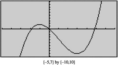
Figure 7.2-12
Example 3
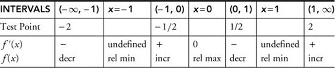
Find the relative extrema for the function f(x) = (x2 − 1)2/3.
Using the First Derivative Test
Step 1: Find f′(x).
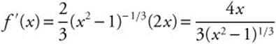
Step 2: Find all critical numbers of f.
Set f′(x) = 0. Thus, 4x = 0 or x = 0.
Set x2 − 1 = 0. Thus, f′(x) is undefined at x = 1 and x = − 1. Therefore, the critical numbers are − 1, 0 and 1.
Step 3: Determine intervals.
![]()
The intervals are (− ∞, − 1), (− 1, 0), (0, 1), and (1, ∞).
Step 4: Set up a table.
Step 5: Write a conclusion.
Using the First Derivative Test, note that f(x) has a relative maximum at x = 0 and relative minimums at x = − 1 and x = 1.
Note that f (− 1) = 0, f (0) = 1, and f (1) = 0. Therefore, 1 is a relative maximum value and 0 is a relative minimum value. (See Figure 7.2-13.)
Figure 7.2-13
• Do not forget the constant, C, when you write the antiderivative after evaluating an indefinite integral, e.g., ∫ cos xdx = sin x + C.
Test for Concavity and Points of Inflection
Test for Concavity
Let f be a differentiable function.
1. If f″ > 0 on an interval I, then f is concave upward on I.
2. If f″ < 0 on an interval I, then f is concave downward on I.
(See Figures 7.2-14 and 7.2-15.)
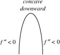
Figure 7.2-14
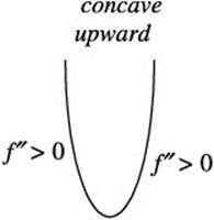
Figure 7.2-15
Points of Inflection
A point P on a curve is a point of inflection if:
1. the curve has a tangent line at P, and
2. the curve changes concavity at P (from concave upward to downward or from concave downward to upward).
(See Figures 7.2-16–7.2-18.)
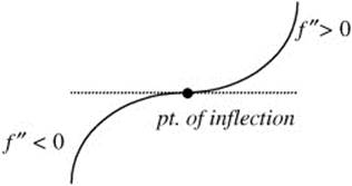
Figure 7.2-16
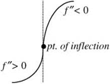
Figure 7.2-17
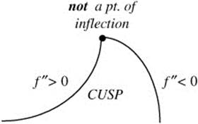
Figure 7.2-18
Note that if a point (a, f(a)) is a point of inflection, then f″(c) = 0 or f″(c) does not exist. (The converse of the statement is not necessarily true.)
Note: There are some textbooks that define a point of inflection as a point where the concavity changes and do not require the existence of a tangent at the point of inflection. In that case, the point at the cusp in Figure 7.2-18would be a point of inflection.
Example 1
The graph of f′, the derivative of a function f, is shown in Figure 7.2-19. Find the points of inflection of f and determine where the function f is concave upward and where it is concave downward on [− 3, 5].
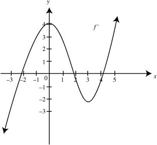
Figure 7.2-19
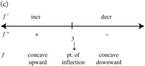
Solution: (See Figure 7.2-20.)
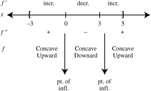
Figure 7.2-20
Thus, f is concave upward on [− 3, 0) and (3, 5], and is concave downward on (0, 3).
There are two points of inflection: one at x = 0 and the other at x = 3.
Example 2
Using a calculator, find the values of x at which the graph of y = x2 ex changes concavity.
Enter y1 = x∧ 2 * e∧x and y2 = d(y1(x), x, 2). The graph of y2, the second derivative of y, is shown in Figure 7.2-21. Using the [Zero] function, you obtain x = − 3.41421 and x = − 0.585786. (See Figures 7.2-21 and 7.2-22.)
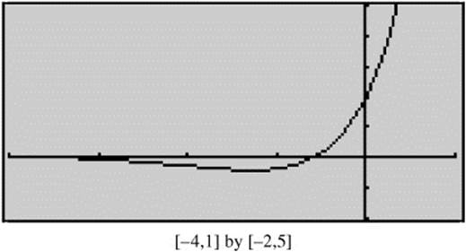
Figure 7.2-21
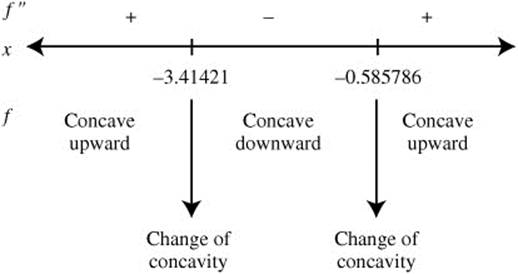
Figure 7.2-22
Thus, f changes concavity at x = − 3.41421 and x = − 0.585786.
Example 3
Find the points of inflection of f(x) = x3 − 6x2 + 12x − 8 and determine the intervals where the function f is concave upward and where it is concave downward.
Step 1: Find f″(x) and f″(x).
f′(x) = 3x2 − 12x + 12
f″(x) = 6x − 12
Step 2: Set f″(x) = 0.
6x − 12 = 0
x = 2
Note that f″(x) is defined for all real numbers.
Step 3: Determine intervals.
![]()
The intervals are (− ∞, 2) and (2, ∞).
Step 4: Set up a table.
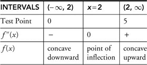
Since f(x) has change of concavity at x = 2, the point (2, f (2)) is a point of inflection. f (2) = (2)3 − 6(2)2 + 12(2) − 8 = 0.
Step 5: Write a conclusion.
Thus, f(x) is concave downward on (− ∞, 2), concave upward on (2, ∞) and f(x) has a point of inflection at (2, 0). (See Figure 7.2-23.)
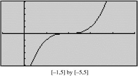
Figure 7.2-23
Example 4
Find the points of inflection of f(x) = (x − 1)2/3 and determine the intervals where the function f is concave upward and where it is concave downward.
Step 1: Find f′(x) and f″(x).
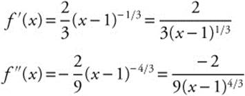
Step 2: Find all values of x where f″(x) = 0 or f″(x) is undefined. Note that f″(x) ≠ 0 and that f″(1) is undefined.
Step 3: Determine intervals.
![]()
The intervals are (− ∞, 1), and (1, ∞).
Step 4: Set up a table.
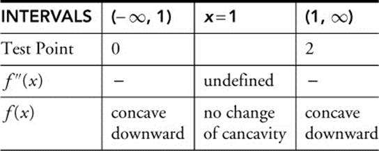
Note that since f(x) has no change of concavity at x = 1, f does not have a point of inflection.
Step 5: Write a conclusion.
Therefore, f(x) is concave downward on (− ∞, ∞) and has no point of inflection. (See Figure 7.2-24.)
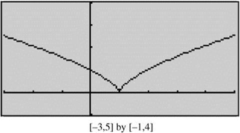
Figure 7.2-24
Example 5
The graph of f is shown in Figure 7.2-25 and f is twice differentiable. Which of the following statements is true?
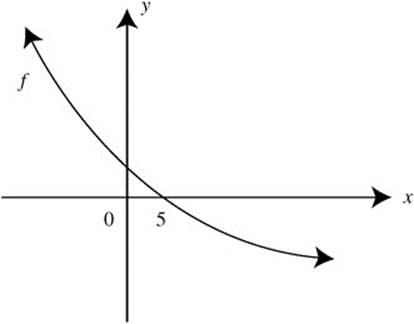
Figure 7.2-25
(A) f(5) < f′(5) < f″(5)
(B) f″(5) < f′(5) < f(5)
(C) f′(5) < f(5) < f″(5)
(D) f′(5) < f″(5) < f(5)
(E) f″(5) < f(5) < f′(5)
The graph indicates that (1) f(5) = 0, (2) f′(5) < 0, since f is decreasing; and (3) f″(5) > 0, since f is concave upward. Thus, f′(5) < f(5) < f″(5), choice (C).
• Move on. Do not linger on a problem too long. Make an educated guess. You can earn many more points from other problems.
7.3 Sketching the Graphs of Functions
Main Concepts:
Graphing without Calculators, Graphing with Calculators
Graphing without Calculators
General Procedure for Sketching the Graph of a Function

Steps:
1. Determine the domain and if possible the range of the function f(x).
2. Determine if the function has any symmetry, i.e., if the function is even (f(x) = f(− x)), odd (f(x) = − f(− x)), or periodic (f(x + p) = f(x)).
3. Find f′(x) and f″(x).
4. Find all critical numbers (f′(x) = 0 or f′(x) is undefined) and possible points of inflection (f″(x) = 0 or f″(x) is undefined).
5. Using the numbers in Step 4, determine the intervals on which to analyze f(x).
6. Set up a table using the intervals, to
(a) determine where f(x) is increasing or decreasing.
(b) find relative and absolute extrema.
(c) find points of inflection.
(d) determine the concavity of f(x) on each interval.
7. Find any horizontal, vertical, or slant asymptotes.
8. If necessary, find the x-intercepts, the y-intercepts, and a few selected points.
9. Sketch the graph.
Example 1
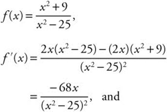
Sketch the graph of ![]() .
.
Step 1: Domain: all real numbers x ≠ ± 5.
Step 2: Symmetry: f(x) is an even function (f(x) = f(−x)); symmetrical with respect to the y-axis.
Step 3:
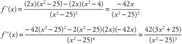
Step 4: Critical numbers:
f′(x) = 0 ⇒ − 42x = 0 or x = 0
f′(x) is undefined at x = ± 5 which are not in the domain. Possible points of inflection:
f″(x) ≠ 0 and f″(x) is undefined at x = ± 5 which are not in the domain.
Step 5: Determine intervals:
![]()
Intervals are (− ∞, − 5), (5, 0), (0, 5) & (5, ∞)
Step 6: Set up a table:
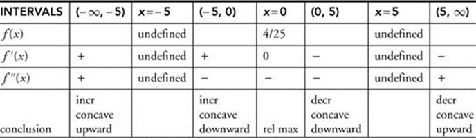
Step 7: Vertical asymptote: x = 5 and x = − 5
Horizontal asymptote: y = 1
Step 8: y-intercept: 
x-intercept: (− 2, 0) and (2, 0) (See Figure 7.3-1.)
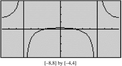
Figure 7.3-1
Graphing with Calculators
Example 1
Using a calculator, sketch the graph of f(x) = − x5/3 + 3x2/3 indicating all relative extrema, points of inflection, horizontal and vertical asymptotes, intervals where f(x) is increasing or decreasing, and intervals where f(x) is concave upward or downward.
1. Domain: all real numbers; Range: all real numbers
2. No symmetry
3. Relative maximum: (1.2, 2.03)
Relative minimum: (0, 0)
Points of inflection: (− 0.6, 2.56)
4. No asymptote
5. f(x) is decreasing on (− ∞, 0], [1.2, ∞) and increasing on (0, 1.2).
6. Evaluating f″(x) on either side of the point of inflection (− 0.6, 2.56)
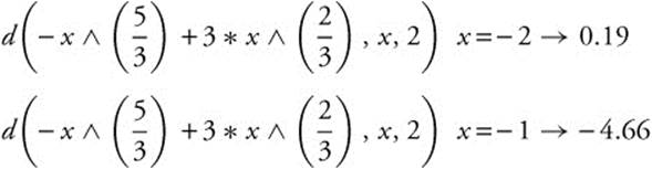
⇒ f(x) is concave upward on (− ∞, − 0.6) and concave downward on (− 0.6, ∞). (See Figure 7.3-2.)
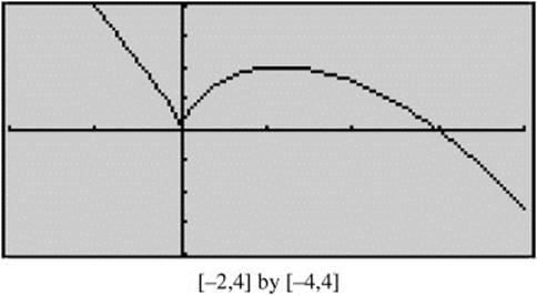
Figure 7.3-2
Example 2
Using a calculator, sketch the graph of f(x) = e−x2/2, indicating all relative minimum and maximum points, points of inflection, vertical and horizontal asymptotes, intervals on which f(x) is increasing, decreasing, concave upward or concave downward.
1. Domain: all real numbers; Range (0, 1]
2. Symmetry: f(x) is an even function, and thus is symmetrical with respect to the y-axis.
3. Relative maximum: (0, 1)
No relative minimum
Points of inflection: (− 1, 0.6) and (1, 0.6)
4. y = 0 is a horizontal asymptote; no vertical asymptote.
5. f(x) is increasing on (− ∞, 0] and decreasing on [0, ∞).
6. f(x) is concave upward on (− ∞, − 1) and (1, ∞); and concave downward on (− 1, 1).
(See Figure 7.3-3.)
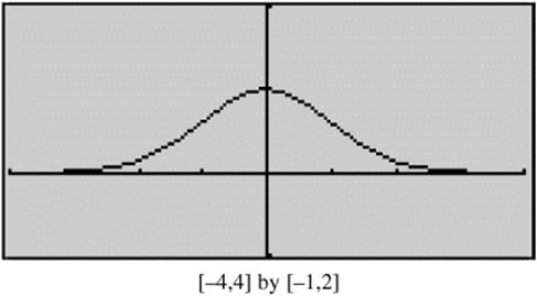
Figure 7.3-3
• When evaluating a definite integral, you do not have to write a constant C, e.g., ![]() . Notice, no C.
. Notice, no C.
7.4 Graphs of Derivatives
The functions f, f′, and f″ are interrelated, and so are their graphs. Therefore, you can usually infer from the graph of one of the three functions (f, f′, or f″) and obtain information about the other two. Here are some examples.
Example 1
The graph of a function f is shown in Figure 7.4-1. Which of the following is true for f on (a, b)?
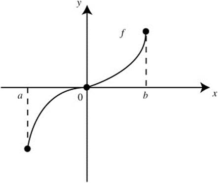
Figure 7.4-1
I. f′ ≥ 0 on (a, b)
II. f″ > 0 on (a, b)
Solution:
I. Since f is strictly increasing, f′ ≥ 0 on (a, b) is true.
II. The graph is concave downward on (a, 0) and upward on (0, b). Thus, f″ > 0 on (0, b) only. Therefore, only statement I is true.
Example 2
Given the graph of f′ in Figure 7.4-2, find where the function f (a) has its relative maximum(s) or relative minimums, (b) is increasing or decreasing, (c) has its point(s) of inflection, (d) is concave upward or downward, and (e) if f(− 2) = f(2) = 1 and f(0) = − 3, draw a sketch of f.
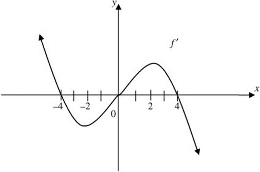
Figure 7.4-2
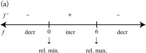
(a) Summarize the information of f′ on a number line:
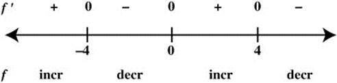
The function f has a relative maximum at x = − 4 and at x = 4, and a relative minimum at x = 0.
(b) The function f is increasing on interval (− ∞, − 4] and [0, 4], and f is decreasing on [− 4, 0] and [4, ∞).
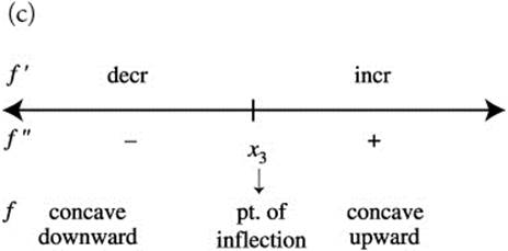
(c) Summarize the information of f″ on a number line:
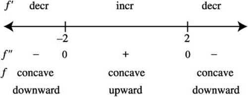
A change of concavity occurs at x = − 2 and at x = 2 and f′ exists at x = − 2 and at x = 2, which implies that there is a tangent line to the graph of f at x = − 2 and at x = 2. Therefore, f has a point of inflection at x = − 2 and at x = 2.
(d) The graph of f is concave upward on the interval (− 2, 2) and concave downward on (− ∞, − 2) and (2, ∞).
(e) A sketch of the graph of f is shown in Figure 7.4-3.
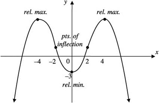
Figure 7.4-3
Example 3
Given the graph of f′ in Figure 7.4-4, find where the function f (a) has a horizontal tangent, (b) has its relative extrema, (c) is increasing or decreasing, (d) has a point of inflection, and (e) is concave upward or downward.
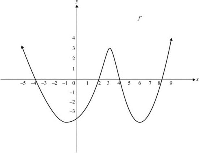
Figure 7.4-4
(a) f′(x) = 0 at x = − 4, 2, 4, 8. Thus, f has a horizontal tangent at these values.
(b) Summarize the information of f′ on a number line:

The First Derivative Test indicates that f has relative maximums at x = − 4 and 4; and f has relative minimums at x = 2 and 8.
(c) The function f is increasing on (− ∞, − 4], [2, 4], and [8, ∞) and is decreasing on [− 4, 2] and [4, 8].
(d) Summarize the information of f″ on a number line:
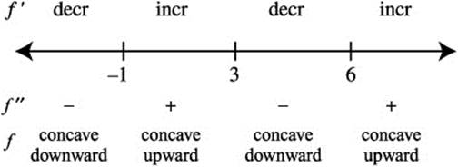
A change of concavity occurs at x = − 1, 3, and 6. Since f′(x) exists, f has a tangent at every point. Therefore, f has a point of inflection at x = − 1, 3, and 6.
(e) The function f is concave upward on (− 1, 3) and (6, ∞) and concave downward on (− ∞, − 1) and (3, 6).
Example 4
A function f is continuous on the interval [− 4, 3] with f (− 4) = 6 and f (3) = 2 and the following properties:
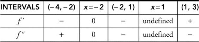
(a) Find the intervals on which f is increasing or decreasing.
(b) Find where f has its absolute extrema.
(c) Find where f has the points of inflection.
(d) Find the intervals where f is concave upward or downward.
(e) Sketch a possible graph of f.
Solution:
(a) The graph of f is increasing on [1, 3] since f′ > 0 and decreasing on [− 4, − 2] and [− 2, 1] since f′ < 0.
(b) At x = − 4, f(x) = 6. The function decreases until x = 1 and increases back to 2 at x = 3. Thus, f has its absolute maximum at x = − 4 and its absolute minimum at x = 1.
(c) A change of concavity occurs at x = − 2, and since f′(− 2) = 0, which implies a tangent line exists at x = − 2, f has a point of inflection at x = − 2.
(d) The graph of f is concave upward on (− 4, − 2) and concave downward on (− 2, 1) and (1, 3).
(e) A possible sketch of f is shown in Figure 7.4-5.
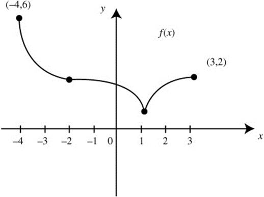
Figure 7.4-5
Example 5
If f(x) =ln(x + 1)|, find ![]() . (See Figure 7.4-6.)
. (See Figure 7.4-6.)
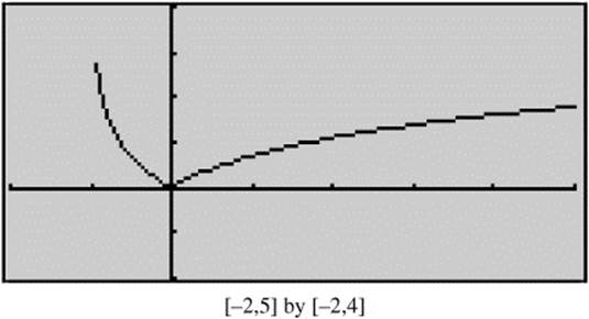
Figure 7.4-6
The domain of f is (− 1, ∞).
f(0) = |ln(0 + 1)| = |ln(1)| = 0
Thus,
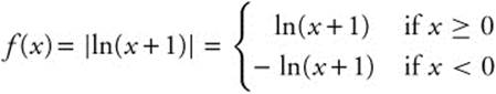
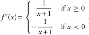
Therefore, 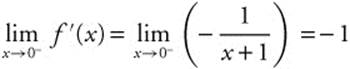 .
.
 7.5 Parametric, Polar, and Vector Representations
Main Concepts:
Parametric Curves, Polar Equations, Types of Polar Graphs, Symmetry of Polar Graphs, Vectors, Vector Arithmetic
Parametric Curves
Parametric curves are relations (x(t), y(t)) for which both x and y are defined as functions of a third variable, t, that is, x = f (t) and y = g (t).
Example 1
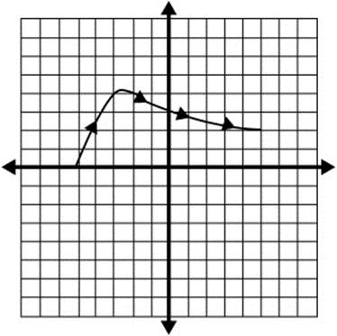
A particle is moving in the coordinate plane in such a way that x(t) = 2t − 5 and ![]() for 0 ≤ t ≤ 5. Sketch the path of the particle and indicate the direction of motion.
for 0 ≤ t ≤ 5. Sketch the path of the particle and indicate the direction of motion.
Step 1: Create a table of values.
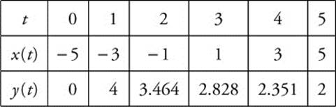
Step 2: Plot the points and sketch the path of a particle as a smooth curve. Place arrows to indicate the direction of motion.
Example 2
A parametric curve is defined by x = 2 + et and y = e3t. Find the Cartesian equation of the curve.
Step 1: Solve x = 2 + et for t. x − 2 = et so t = ln(x − 2).
Step 2: Substitute t = ln(x − 2) into y = e3t. y = e3 ln(x − 2) = (x − 2)3.
Step 3: Note that t = ln(x − 2) is defined only when x > 2. The equation of the curve is y = (x − 2)3 with domain (2, ∞).
Polar Equations
The polar coordinate system locates points by a distance from the origin or pole, and an angle of rotation. Points are represented by a coordinate pair (r, θ). If conversions between polar and Cartesian representations are necessary, make the appropriate substitutions and simplify.
![]()
Example 1
Convert r = 4 sinθ to Cartesian coordinates.
Step 1: Substitute in r = 4 sinθ to get ![]() .
.
Step 2: Since ![]() , this becomes
, this becomes ![]() .
.
Multiplying through by ![]() , gives x2 + y2 = 4y.
, gives x2 + y2 = 4y.
Step 3: Complete the square on x2 + y2 − 4y = 0 to produce x2 + (y − 2)2 = 4.
Example 2
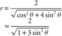
Find the polar representation of ![]() .
.
Step 1: Substitute in ![]() to produce
to produce ![]() .
.
Step 2: Simplify and clear denominators to get 9r2 cos2 θ + 4r2 sin2 θ = 36, then factor for r2(9 cos2 θ + 4 sin2 θ) = 36.
Step 3: Divide to isolate ![]() .
.
Step 4: Apply the Pythagorean identity to the denominator ![]() .
.
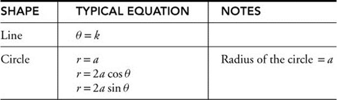
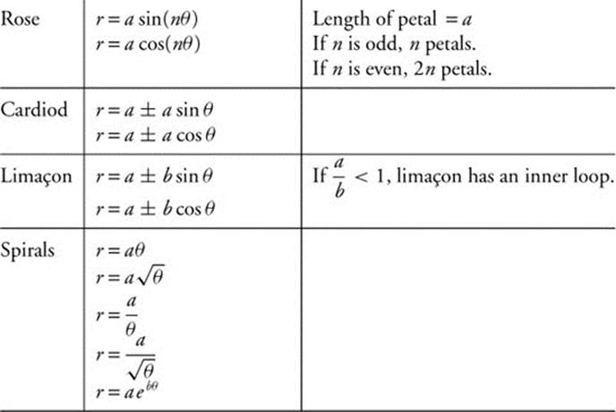
Types of Polar Graphs
Example 1
Classify each of the following equations according to the shape of its graph. (a) r = 5 + 7 cos θ, ![]() , (c) r = 4 − 4 sin θ.
, (c) r = 4 − 4 sin θ.
The equation in (a) is a limaçon, and since ![]() , it will have an inner loop. The equation in (b) is a spiral. Equation (c) appears at first glance to be a limaçon; however, since the coefficients are equal, it is a cardiod.
, it will have an inner loop. The equation in (b) is a spiral. Equation (c) appears at first glance to be a limaçon; however, since the coefficients are equal, it is a cardiod.
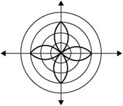
Example 2
Sketch the graph of r = 3 cos(2θ). The equation r = 3 cos (2θ) is a polar rose with four petals each 3 units long. Since 3 cos(0) = 3, the tip of a petal sits at 3 on the polar axis.
Symmetry of Polar Graphs
A polar curve of the form r = f(θ) will be symmetric about the polar, or horizontal, axis if f(θ) = f(− θ), symmetric about the line ![]() if f(θ) = f(π − θ), and symmetric about the pole if f(θ) = f(θ + π).
if f(θ) = f(π − θ), and symmetric about the pole if f(θ) = f(θ + π).
Example 1
Determine the symmetry, if any, of the graph of r = 2 + 4 cos θ.
Step 1: Since 2 + 4 cos(− θ) = 2 + 4 cos θ, the graph is symmetric about the polar axis.
Step 2: 2 + 4 cos(π − θ) = 2 − 4 cos θ, so the graph is not symmetric about the line ![]() .
.
Step 3: Since 2 + 4 cos(θ + π) = 2 + 4 [cos θ cos π − sinθ sin π] = 2 − 4 cos θ, the graph is not symmetric about the pole.
Example 2
Determine the symmetry, if any, of the graph r = 3 − 3 sinθ.
Step 1: Since 3 − 3 sin(− θ) = 3 + 3 sinθ is not equal to r = 3 − 3 sinθ, the graph is not symmetric about the polar axis.
Step 2: 3 − 3 sin(π − θ) = 3 − 3 sinθ, so the graph is symmetric about the line θ = π/2.
Step 3: Since 3 − 3 sin(θ + π) = 3 − 3[sinθ cos π + sin π cos θ] = 3 + 3 sinθ, the graph is not symmetric about the pole.
Example 3
Determine the symmetry, if any, of the graph of r = 5 cos(4θ).
Step 1: Since 5 cos(4(− θ)) = 5 cos 4θ, the graph is symmetric about the polar axis.
Step 2: 5 cos(4(π − θ)) = 5 cos(4π − 4θ) which, by identity, is equal to 5[cos 4π cos 4θ + sin 4π sinθ] or 5 cos 4θ, the graph is symmetric about the line θ = π/2.
Step 3: Since 5 cos 4(θ + π) = 5 cos(4θ + 4π) = 5 cos(4θ), the graph is symmetric about the pole.
Vectors
A vector represents a displacement of both magnitude and direction. The length, r, of the vector is its magnitude, and the angle, θ, it makes with the x-axis gives its direction. The vector can be resolved into a horizontal and a vertical component. x = ||r|| cos θ and y = ||r|| sinθ.
A unit vector is a vector of magnitude 1. If i = ⟨1, 0⟩ is the unit vector parallel to the positive x-axis, that is, a unit vector with direction angle θ = 0, and j = ⟨0, 1⟩ is the unit vector parallel to the y-axis, with an angle ![]() , then any vector in the plane can be represented as xi + yj or simply as the ordered pair ⟨x, y⟩. The magnitude of the vector is
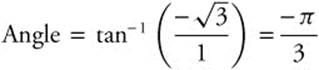
, then any vector in the plane can be represented as xi + yj or simply as the ordered pair ⟨x, y⟩. The magnitude of the vector is ![]() , and the direction can be found from tan
, and the direction can be found from tan ![]() . Since
. Since ![]() will return values in quadrant I or quadrant IV, if the terminal point of the vector falls in quadrant II or quadrant III, the direction angle will be equal to
will return values in quadrant I or quadrant IV, if the terminal point of the vector falls in quadrant II or quadrant III, the direction angle will be equal to ![]() .
.
Example 1
Find the magnitude and direction of the vector represented by ⟨6, − 3⟩.
Step 1: Calculate the magnitude ![]() .
.
Step 2: The terminal point of the vector is in the fourth quadrant. Calculate 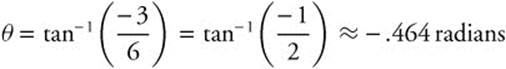 . This angle falls in quadrant IV.
Example 2
Find the magnitude and direction of the vector represented by ⟨− 5, − 5⟩.
Step 1: Calculate the magnitude ![]()
Step 2: The terminal point of the vector is in the third quadrant. Calculate  radians. The direction angle is
 ![]() .
.
Example 3
Find the magnitude and direction of the vector represented by ![]() .
.
Step 1: Calculate the magnitude ![]() .
.
Step 2: The terminal point of the vector is in the second quadrant. Calculate  radians. The direction angle is
 ![]() .
.
Example 4
Find the ordered pair representation of a vector of magnitude 12 and direction ![]() .
. ![]() and
and ![]() so the vector is
so the vector is ![]() .
.
Vector Arithmetic
If C is a constant, r1 = ⟨x1, y1⟩ and r2 = ⟨x2, y2⟩, then:
Addition: r1 + r2 = ⟨x1 + x2, y1 + y2⟩
Subtraction: r1 − r2 = ⟨x1 − x2, y1 − y2⟩
Scalar Multiplication: Cr1 = ⟨Cx1, Cy1⟩
Note: ||Cr1|| = ||C|| · ||r1||
Dot Product: The dot product of two vectors is r1 · r2 = ||r1|| · ||r2|| · cos θ or r1 · r2 = x1x2 + y1y2.
Parallel and Perpendicular Vectors
If r2 = Cr1, then r1 and r2 are parallel.
If r1 · r2 = 0, then r1 and r2 are perpendicular or orthogonal.
The angle between two vectors can be found by ![]() .
.
Example 1
Given r1 = ⟨4, − 7⟩, r2 = ⟨− 3, − 2⟩ and r2 = ⟨− 1, 5⟩, find 3r1 − 5r2 + 2r3.
3r1 − 5r2 − 2r3 = 3 ⟨4, − 7⟩ − 5 ⟨− 3, − 2⟩ + 2 ⟨ − 1, 5⟩ = ⟨12, − 21⟩ − ⟨− 15, − 10⟩ + ⟨− 2, 10⟩ = ⟨27, − 11⟩ − ⟨− 2, 10⟩ = ⟨29, − 21⟩.
Example 2
Determine whether the vectors r1 = ⟨4, − 7⟩ and r2 = ⟨− 3, − 2⟩ are orthogonal. If the vectors are not orthogonal, approximate the angle between them.
Step 1. Find the dot product r1 · r2 = 4(− 3) + (− 7)(− 2) = 2. Since the dot product is not equal to zero, the vectors are not orthogonal.
Step 2. If θ is the angle between the vectors, then ![]() . The dot product is
. The dot product is ![]() , and
, and ![]() , so
, so  and θ ≈ 1.5019 radians.
7.6 Rapid Review
1. If f′(x) = x2 − 4, find the intervals where f is decreasing. (See Figure 7.6-1.)
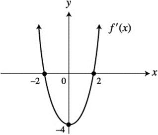
Figure 7.6-1
Answer: Since f′(x) < 0 if − 2 < x < 2, f is decreasing on (− 2, 2).
2. If f″(x) = 2x − 6 and f′ is continuous, find the values of x where f has a point of inflection. (See Figure 7.6-2.)
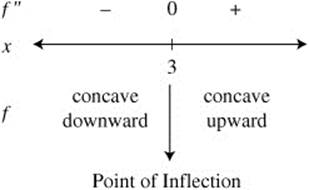
Figure 7.6-2
Answer: Thus, f has a point of inflection at x = 3.
3. (See Figure 7.6-3.) Find the values of x where f has change of concavity.
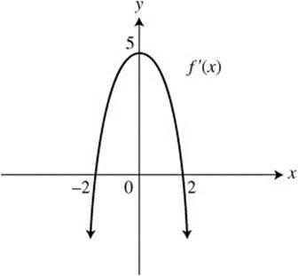
Figure 7.6-3
Answer: f has a change of concavity at x = 0. (See Figure 7.6-4.)
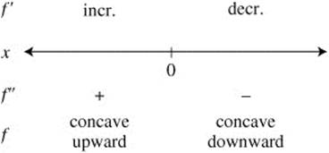
Figure 7.6-4
4. (See Figure 7.6-5.) Find the values of x where f has a relative minimum.
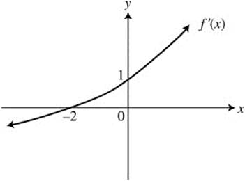
Figure 7.6-5
Answer: f has a relative minimum at x = − 2. (See Figure 7.6-6.)
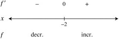
Figure 7.6-6
5. (See Figure 7.6-7.) Given f is twice differentiable, arrange f(10), f′(10), f″(10) from smallest to largest.
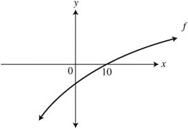
Figure 7.6-7
Answer: f(10) = 0, f′(10) > 0 since f is increasing, and f″(10) < 0 since f is concave downward. Thus, the order is f″(10), f(10), f′(10).
6. (See Figure 7.6-8.) Find the values of x where f″ is concave up.
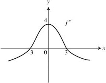
Figure 7.6-8
Answer: f′ is concave upward on (− ∞, 0). (See Figure 7.6-9.)
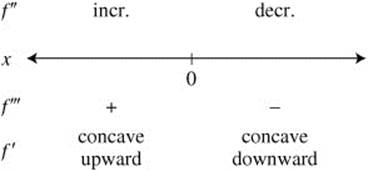
Figure 7.6-9
7. The path of an object is defined by x = 2t, y = t + 1. Find the location of the object when t = 5.
Answer: When t = 5, x = 2(5) = 10 and y = 5 + 1 = 6 so the location is (10, 6).
8. Identify the shape of each equation: ![]() ; (b) r = 6 cos 3θ
; (b) r = 6 cos 3θ
Answers: (a) spiral, (b) rose
9. Find the magnitude of the vector ![]() and the angle it makes with the positive x-axis.
and the angle it makes with the positive x-axis.
Answers: ![]() .
.
 .
.
10. If a = ⟨4, − 2⟩, b = ⟨− 3, 1⟩, and c = ⟨0, 5⟩, find 3a − 2b + c.
Answer: 3⟨4, − 2⟩ − 2⟨− 3, 1⟩ + ⟨0, 5⟩ = ⟨12, − 6⟩ + ⟨6, − 2⟩ + ⟨0, 5⟩ = ⟨18, − 8⟩ + ⟨0, 5⟩ = ⟨18, − 3⟩.
7.7 Practice Problems
Part A—The use of a calculator is not allowed.
1. If f(x) = x3 − x2 − 2x, show that the hypotheses of Rolle’s Theorem are satisfied on the interval [− 1, 2] and find all values of c that satisfy the conclusion of the theorem.
2. Let f(x) = ex. Show that the hypotheses of the Mean Value Theorem are satisfied on [0, 1] and find all values of c that satisfy the conclusion of the theorem.
3. Determine the intervals in which the graph of ![]() is concave upward or downward.
is concave upward or downward.
4. Given f(x) = x + sin x 0 ≤ x ≤ 2π, find all points of inflection of f.
5. Show that the absolute minimum of ![]() on [− 5, 5] is 0 and the absolute maximum is 5.
on [− 5, 5] is 0 and the absolute maximum is 5.
6. Given the function f in Figure 7.7-1, identify the points where:
(a) f′ < 0 and f″ > 0,
(b) f′ < 0 and f″ < 0,
(c) f′ = 0,
(d) f″ does not exist.
7. Given the graph of f″ in Figure 7.7-2, determine the values of x at which the function f has a point of inflection. (See Figure 7.7-2.)
8. If f″(x) = x2(x + 3)(x − 5), find the values of x at which the graph of f has a change of concavity.
9. The graph of f′ on [− 3, 3] is shown in Figure 7.7-3. Find the values of x on [− 3, 3] such that (a) f is increasing and (b) f is concave downward.
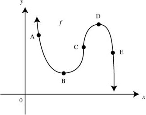
Figure 7.7-1
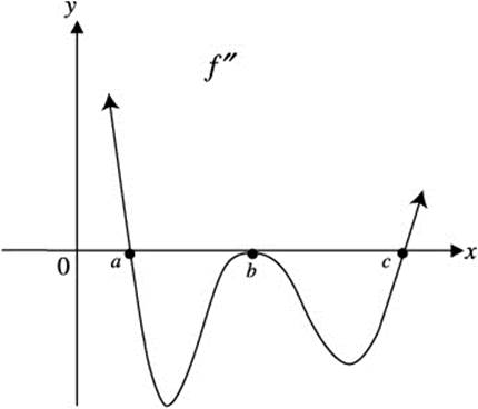
Figure 7.7-2
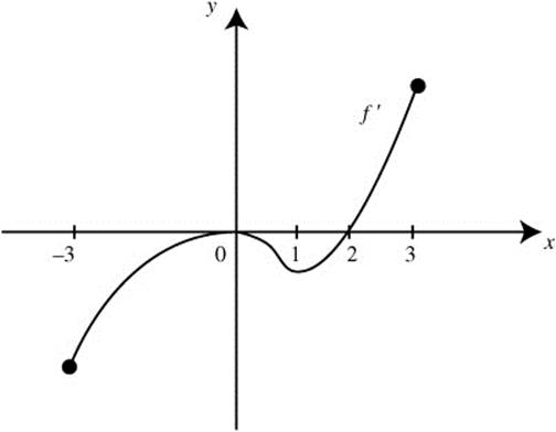
Figure 7.7-3
10. The graph of f is shown in Figure 7.7-4 and f is twice differentiable. Which of the following has the largest value:
(A) f (− 1)
(B) f′(− 1)
(C) f″(− 1)
(D) f (− 1) and f′(− 1)
(E) f′(− 1) and f″(− 1)
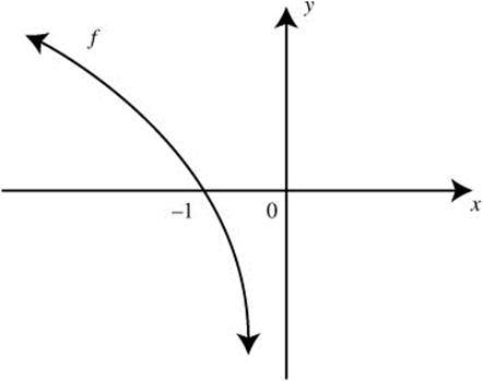
Figure 7.7-4
Sketch the graphs of the following functions indicating any relative and absolute extrema, points of inflection, intervals on which the function is increasing, decreasing, concave upward or concave downward.
11. f(x) = x4 − x2
12. ![]()
Part B Calculators are allowed.
13. Given the graph of f″ in Figure 7.7-5, determine at which of the four values of x (x1, x2, x3, x4) f has:
(a) the largest value,
(b) the smallest value,
(c) a point of inflection,
(d) and at which of the four values of x does f″ have the largest value.
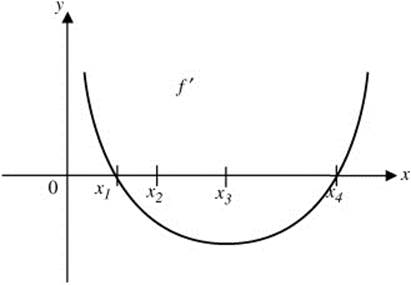
Figure 7.7-5
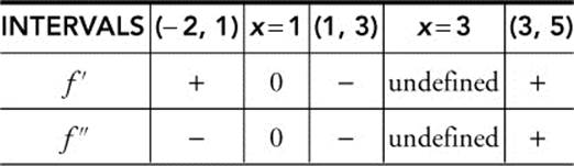
14. Given the graph of f in Figure 7.7-6, determine at which values of x is
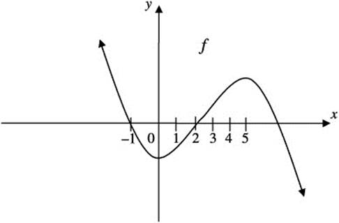
Figure 7.7-6
(a) f′(x) = 0
(b) f″(x) = 0
(c) f′ a decreasing function.
15. A function f is continuous on the interval [− 2, 5] with f (− 2) = 10 and f(5) = 6 and the following properties:
(a) Find the intervals on which f is increasing or decreasing.
(b) Find where f has its absolute extrema.
(c) Find where f has points of inflection.
(d) Find the intervals where f is concave upward or downward.
(e) Sketch a possible graph of f.
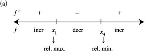
16. Given the graph of f′ in Figure 7.7-7, find where the function f
(a) has its relative extrema.
(b) is increasing or decreasing.
(c) has its point(s) of inflection.
(d) is concave upward or downward.
(e) if f(0) = 1 and f(6) = 5, draw a sketch of f.
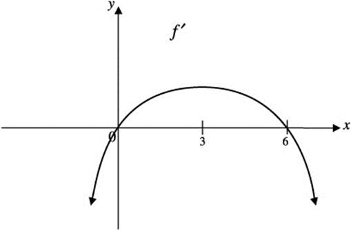
Figure 7.7-7
17. If f(x) = |x2 − 6x − 7|, which of the following statements about f are true?
I. f has a relative maximum at x = 3.
II. f is differentiable at x = 7.
III. f has a point of inflection at x = − 1.
18. How many points of inflection does the graph of y = cos(x2) have on the interval [− π, π]?
Sketch the graphs of the following functions indicating any relative extrema, points of inflection, asymptotes, and intervals where the function is increasing, decreasing, concave upward or concave downward.
19. f(x) = 3e−x2/2
20. f(x) = cos x sin2 x [0, 2π]
21. Find the Cartesian equation of the curve defined by ![]() , y = t2 − 4t + 1.
, y = t2 − 4t + 1.
22. Find the polar equation of the line with Cartesian equation y = 3x − 5.
23. Identify the type of graph defined by the equation r = 2 − sinθ and determine its symmetry, if any.
24. Find the value of k so that the vectors ⟨3, − 2⟩ and ⟨1, k⟩ are orthogonal.
25. Determine whether the vectors ⟨5, − 3⟩ and ⟨5, 3⟩ are orthogonal. If not, find the angle between the vectors.
7.8 Cumulative Review Problems
(Calculator) indicates that calculators are permitted.
26. Find ![]() .
.
27. Evaluate  .
.
28. Find ![]() .
.
29. (Calculator) Determine the value of k such that the function 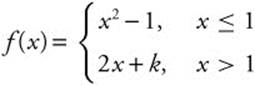 is continuous for all real numbers.
30. A function f is continuous on the interval [− 1, 4] with f (− 1) = 0 and f (4) = 2 and the following properties:
(a) Find the intervals on which f is increasing or decreasing.
(b) Find where f has its absolute extrema.
(c) Find where f has points of inflection.
(d) Find intervals on which f is concave upward or downward.
(e) Sketch a possible graph of f.
31. Evaluate ![]() .
.
32. Evaluate  .
.
33. Find the polar equation of the ellipse x2 + 4y2 = 4.
7.9 Solutions to Practice Problems
Part A—The use of a calculator is not allowed.
1. Condition 1: Since f(x) is a polynomial, it is continuous on [− 1, 2].
Condition 2: Also, f(x) is differentiable on (− 1, 2) because f′(x) = 3x2 − 2x − 2 is defined for all numbers in [− 1, 2].
Condition 3: f (− 1) = f(2) = 0. Thus, f(x) satisfies the hypotheses of Rolle’s Theorem which means there exists a c in [− 1, 2] such that f′(c) = 0. Set f′(x) = 3x2 − 2x − 2 = 0. Solve 3x2 − 2x − 2 = 0, using the quadratic formula and obtain  . Thus, x ≈ 1.215 or − 0.549 and both values are in the interval (− 1, 2). Therefore,
  .
.
2. Condition 1: f(x) = ex is continuous on [0, 1].
Condition 2: f(x) is differentiable on (0, 1) since f′(x) = ex is defined for all numbers in [0, 1].
Thus, there exists a number c in [0, 1] such that ![]() . Set f′(x) = ex = (e − 1). Thus, ex = (e − 1). Take ln of both sides. ln(ex) = ln(e − 1) ⇒ x = ln(e − 1). Thus, x ≈ 0.541 which is in the interval (0, 1). Therefore, c = ln(e − 1).
. Set f′(x) = ex = (e − 1). Thus, ex = (e − 1). Take ln of both sides. ln(ex) = ln(e − 1) ⇒ x = ln(e − 1). Thus, x ≈ 0.541 which is in the interval (0, 1). Therefore, c = ln(e − 1).
3.
Set f″ > 0. Since (3x2 + 25) > 0, ⇒ (x2 − 25)3 > 0 ⇒ x2 − 25 > 0, x < − 5 or x > 5. Thus, f(x) is concave upward on (− ∞, − 5) and (5, ∞) and concave downward on (− 5, 5).
4. Step 1: f(x) = x + sin x,
f′(x) = 1 + cos x,
f″ = − sin x.
Step 2: Set f″(x) = 0 ⇒ − sin x = 0 or x = 0, π,2π.
Step 3: Check intervals.
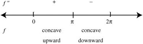
Step 4: Check for tangent line: At x = π, f′(x) = 1 + (− 1) ⇒ 0 there is a tangent line at x = π.
Step 5: Thus, (π, π) is a point of inflection.
5. Step 1: Rewrite f(x) as f(x) = (25 − x2)1/2.
Step 2:
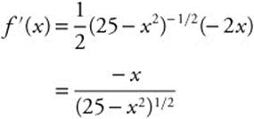
Step 3: Find critical numbers. f′(x) = 0; at x = 0; and f′(x) is undefined at x = ± 5.
Step 4:
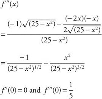
(and f (0) = 5) ⇒ (0, 5) is a relative maximum. Since f(x) is continuous on [− 5, 5], f(x) has both a maximum and a minimum value on [− 5, 5] by the Extreme Value Theorem. And since the point (0,5) is the only relative extremum, it is an absolute extramum. Thus, (0,5) is an absolute maximum point and 5 is the maximum value. Now we check the end points, f (− 5) = 0 and f(5) = 0. Therefore, (− 5, 0) and (5, 0) are the lowest points for f on [− 5, 5]. Thus, 0 is the absolute minimum value.
6. (a) Point A f′ < 0 ⇒ decreasing and f″ > 0 ⇒ concave upward.
(b) Point E f′ < 0 ⇒ decreasing and f″ < 0 ⇒ concave downward.
(c) Points B and D f′ = 0 ⇒ horizontal tangent.
(d) Point C f″ does not exist ⇒ vertical tangent.
7. A change in concavity ⇒ a point of inflection. At x = a, there is a change of concavity; f″ goes from positive to negative ⇒ concavity changes from upward to downward. At x = c, there is a change of concavity; f″ goes from negative to positive ⇒ concavity changes from downward to upward. Therefore, f has two points of inflection, one at x = a and the other at x = c.
8. Set f″(x) = 0. Thus, x2(x + 3)(x − 5) = 0 ⇒ x = 0, x = − 3 or x = 5. (See Figure 7.9-1.)
Thus, f has a change of concavity at x = − 3 and at x = 5.
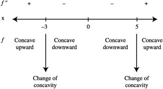
Figure 7.9-1
9. (See Figure 7.9-2.) Thus, f is increasing on [2, 3] and concave downward on (0, 1).
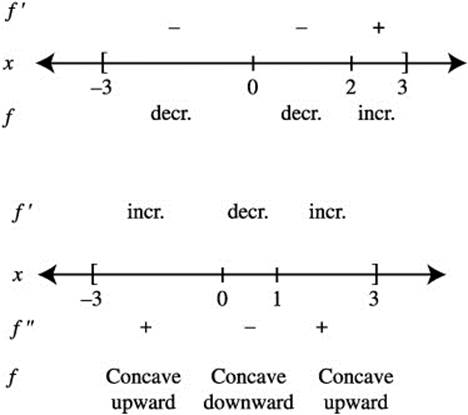
Figure 7.9-2
10. The correct answer is (A).
f (− 1) = 0; f′(0) < 0 since f is decreasing and f″(− 1) < 0 since f is concave downward. Thus, f (− 1) has the largest value.
11. Step 1: Domain: all real numbers.
Step 2: Symmetry: Even function (f(x) = f (− x)); symmetrical with respect to the y-axis.
Step 3: f′(x) = 4x3 − 2x and f″(x) = 12x2 − 2.
Step 4: Critical numbers:
f′(x) is defined for all real numbers. Set f′(x) = 4x3 − 2x = 0 ⇒ 2x (2x2 − 1) = 0 ⇒ x = 0 or ![]() . Possible points of inflection: f″(x) is defined for all real numbers. Set f″(x) = 12x2 − 2 = 0 ⇒
. Possible points of inflection: f″(x) is defined for all real numbers. Set f″(x) = 12x2 − 2 = 0 ⇒ ![]() .
.
Step 5: Determine intervals:
![]()
Intervals are: ![]() ,
, ![]() ,
, ![]() ,
, ![]() , and
, and ![]() .
.
Since f′(x) is symmetrical with respect to the y-axis, you only need to examine half of the intervals.
Step 6: Set up a table (Table 7.9-1). The function has an absolute minimum value of (− 1/4) and no absolute maximum value.
Table 7.9-1
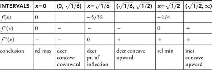
Step 7: Sketch the graph. (See Figure 7.9-3.)
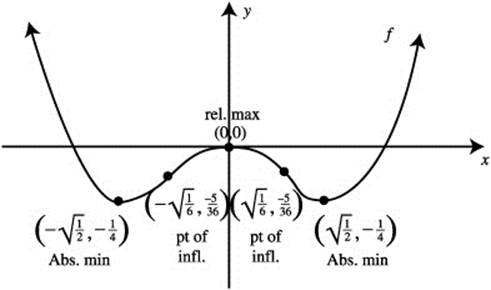
Figure 7.9-3
12. Step 1: Domain: all real numbers x ≠ 4.
Step 2: Symmetry: none.
Step 3: Find f′ and f″.
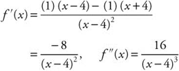
Step 4: Critical numbers: f′(x) ≠ 0 and f′(x) is undefined at x = 4.
Step 5: Determine intervals.
![]()
Intervals are (− ∞, 4) and (4, ∞).
Step 6: Set up table as below:
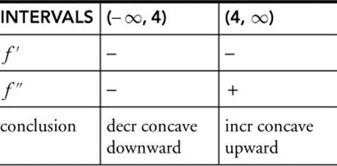
Step 7: Horizontal asymptote:
![]() . Thus, y = 1 is a horizontal asymptote.
. Thus, y = 1 is a horizontal asymptote.
Vertical asymptote: ![]() and
and ![]() ; Thus, x = 4 is a vertical asymptote.
; Thus, x = 4 is a vertical asymptote.
Step 8: x-intercept: Set f′(x) = 0 ⇒ x + 4 = 0; x = − 4. y-intercept: Set x = 0 ⇒ f(x) = − 1.
Step 9: Sketch the graph. (See Figure 7.9-4.)
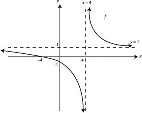
Figure 7.9-4
13.
The function f has the largest value (of the four choices) at x = x1. (See Figure 7.9-5.)
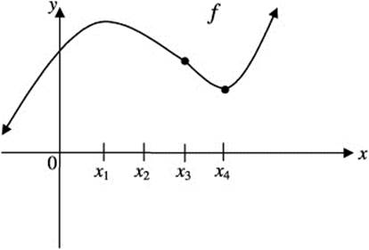
Figure 7.9-5
(b) And f has the smallest value at x = x4.
A change of concavity occurs at x = x3, and f′(x3) exists which implies there is a tangent to f at x = x3. Thus, at x = x3, f has a point of inflection.
(d) The function f″ represents the slope of the tangent to f′. The slope of the tangent to f′ is the largest at x = x4.
14. (a) Since f′(x) represents the slope of the tangent, f′(x) = 0 at x = 0, and x = 5.
(b) At x = 2, f has a point of inflection which implies that if f″(x) exists, f″(x) = 0. Since f′(x) is differentiable for all numbers in the domain, f″(x) exists, and f″(x) = 0 at x = 2.
(c) Since the function f is concave downwards on (2, ∞), f″ < 0 on (2, ∞) which implies f′ is decreasing on (2, ∞).
15. (a) The function f is increasing on the intervals (− 2, 1) and (3, 5) and decreasing on (1, 3).
(b) The absolute maximum occurs at x = 1, since it is a relative maximum, f (1) > f (− 2) and f(5) < f (− 2). Similarly, the absolute minimum occurs at x = 3, since it is a relative minimum, and f (3) < f(5) < f (− 2).
(c) No point of inflection. (Note that at x = 3, f has a cusp.)
Note: Some textbooks define a point of inflection as a point where the concavity changes and do not require the existence of a tangent. In that case, at x = 3, f has a point of inflection.
(d) Concave upward on (3, 5) and concave downward on (− 2, 3).
(e) A possible graph is shown in Figure 7.9-6.
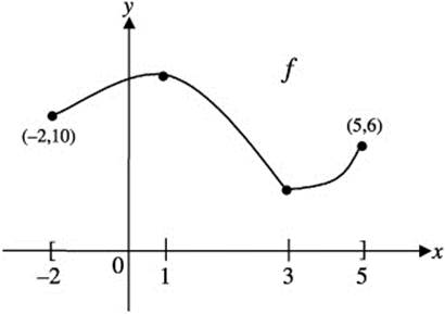
Figure 7.9-6
16.
The function f has its relative minimum at x = 0 and its relative maximum at x = 6.
(b) The function f is increasing on [0, 6] and decreasing on (− ∞,0] and [6, ∞).
Since f′(3) exists and a change of concavity occurs at x = 3, f has a point of inflection at x = 3.
(d) Concave upward on (− ∞,3) and downward on (3, ∞).
(e) Sketch a graph. (See Figure 7.9-7.)
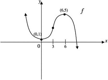
Figure 7.9-7
17. (See Figure 7.9-8.)
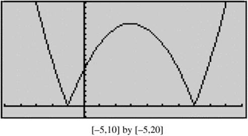
Figure 7.9-8
The graph of f indicates that a relative maximum occurs at x = 3, f is not differentiable at x = 7, since there is a cusp at x = 7 and f does not have a point of inflection at x = − 1, since there is no tangent line at x = − 1. Thus, only statement I is true.
18. (See Figure 7.9-9.)
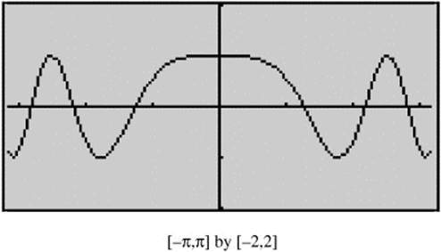
Figure 7.9-9
Enter y1 = cos(x2)
Using the [Inflection] function of your calculator, you obtain three points of inflection on [0, π]. The points of inflection occur at x = 1.35521, 2.1945, and 2.81373. Since y1 = cos(x2), is an even function; there is a total of 6 points of inflection on [− π, π]. An alternate solution is to enter ![]() . The graph of y2 indicates that there are 6 zeros on [− π, π].
. The graph of y2 indicates that there are 6 zeros on [− π, π].
19. Enter y1 = 3 * e ∧ (− x ∧ 2/2). Note that the graph has a symmetry about the y-axis. Using the functions of the calculator, you will find:
(a) a relative maximum point at (0, 3), which is also the absolute maximum point;
(b) points of inflection at (− 1, 1.819) and (1, 1.819);
(c) y = 0 (the x-axis) a horizontal asymptote;
(d) y1 increasing on (− ∞, 0] and decreasing on [0, ∞); and
(e) y1 concave upward on (− ∞, − 1) and (1, ∞) and concave downward on (− 1, 1). (See Figure 7.9-10 on page 148.)
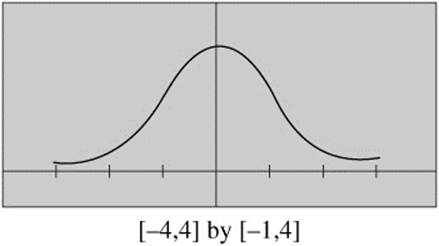
Figure 7.9-10
20. (See Figure 7.9-11.) Enter y1 = cos(x) * (sin(x)) ∧ 2. A fundamental domain of y1 is [0, 2π]. Using the functions of the calculator, you will find:
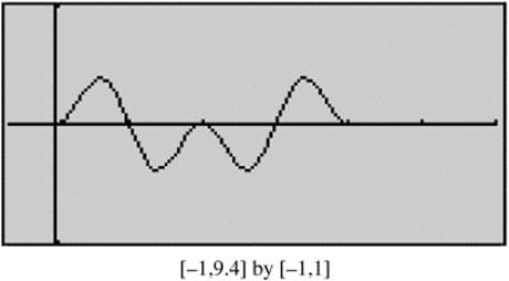
Figure 7.9-11
(a) relative maximum points at (0.955, 0.385), (π, 0) and (5.328, 0.385), and relative minimum points at (2.186, − 0.385) and (4.097, − 0.385);
(b) points of inflection at (0.491, 0.196), ![]() , (2.651, − 0.196), (3.632, − 0.196,
, (2.651, − 0.196), (3.632, − 0.196,  , and (5.792, 0.196);
(c) no asymptote;
(d) function is increasing on intervals (0, 0.955), (2.186, π), and (4.097, 5.328), and decreasing on intervals (0.955, 2.186), (π, 4.097), and (5.328, 2π);
(e) function is concave upward on intervals (0, 0.491), ![]() ,
,  , and (5.792, 2π), and concave downward on the intervals
 ![]() , (2.651, 3.632), and
, (2.651, 3.632), and  .
.
21. Solve ![]() for t = 2x and substitute into y = t2 − 4t + 1. y = (2x)2 − 4(2x) + 1 = 4x2 − 8x + 1.
for t = 2x and substitute into y = t2 − 4t + 1. y = (2x)2 − 4(2x) + 1 = 4x2 − 8x + 1.
22. Since x = r cos θ and y = r sinθ, y = 3x − 5 becomes r sinθ = 3r cos θ − 5. Solving for r produces r (sinθ − 3 cos θ) = − 5 and ![]() .
.
23. The equation r = 2 − sinθ is of the form r = a − b sinθ with ![]() , so the graph is a limaçon with no inner loop. Since r (− θ) = 2 + sinθ ≠ r (θ), the graph is not symmetric about the polar axis. However, r (π − θ) = 2 − sin (π − θ) is equal to 2 sinθ = r (θ), so the graph is symmetric about the line
, so the graph is a limaçon with no inner loop. Since r (− θ) = 2 + sinθ ≠ r (θ), the graph is not symmetric about the polar axis. However, r (π − θ) = 2 − sin (π − θ) is equal to 2 sinθ = r (θ), so the graph is symmetric about the line ![]() . Finally, r(θ + π) = 2 − sin(θ + π) = 2 + sinθ and so the graph is not symmetric about the pole.
. Finally, r(θ + π) = 2 − sin(θ + π) = 2 + sinθ and so the graph is not symmetric about the pole.
24. The vectors ⟨3, − 2⟩ and ⟨1, k⟩ will be orthogonal if the dot product is equal to zero. ⟨3, − 2⟩ · ⟨1, k⟩ = 3.1 − 2k will be equal to zero when 2k = 3 so ![]() .
.
25. The dot product of ⟨5, − 3⟩ and ⟨5, 3⟩ is 5 · 5 + − 3 · 3 = 25 − 9 = 16, so the vectors are not orthogonal. To find the angle between the vectors, begin by dividing the dot product by the product of the magnitudes of the two vectors. Both vectors have a magnitude of ![]() , so the quotient becomes
, so the quotient becomes ![]() . The angle between the vectors is
. The angle between the vectors is  .
.
7.10 Solutions to Cumulative Review Problems
26. (x2 + y2)2 = 10xy
27.
28.
29. (Calculator) The function f is continuous everywhere for all values of k except possibly at x = 1. Checking with the three conditions of continuity at x = 1:
(1) f (1) = (1)2 − 1 = 0
(2) ![]() ,
, ![]() ; thus, 2 + k = 0 ⇒ k = −2. Since
; thus, 2 + k = 0 ⇒ k = −2. Since ![]() , therefore,
, therefore, ![]() .
.
(3) ![]() . Thus, k = −2.
. Thus, k = −2.
30. (a) Since f′ > 0 on (− 1, 0) and (0, 2), the function f is increasing on the intervals [− 1, 0] and [0, 2]. Since f′ < 0 on (2, 4), f is decreasing on [2, 4].
(b) The absolute maximum occurs at x = 2, since it is a relative maximum and it is the only relative extremum on (− 1, 4). The absolute minimum occurs at x = − 1, since f (− 1) < f (4) and the function has no relative minimum on [− 1, 4].
(c) A change of concavity occurs at x = 0. However, f′(0) is undefined, which implies f may or may not have a tangent at x = 0. Thus, f may or may not have a point of inflection at x = 0.
(d) Concave upward on (− 1, 0) and concave downward on (0, 4).
(e) A possible graph is shown in Figure 7.10-1 on page 150.
31. ![]() . Note that L’Hôpital’s Rule does not apply, since the form is not
. Note that L’Hôpital’s Rule does not apply, since the form is not ![]() .
. ![]() but
but ![]() ; therefore,
; therefore, ![]() does not exist.
does not exist.
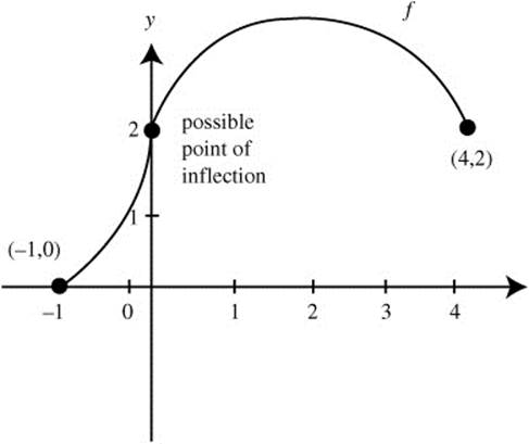
Figure 7.10-1
32.  , but by L’Hôpital’s Rule
33. To convert x2 + 4y2 = 4 to a polar representation, recall that x = r cos θ and y = r sinθ. Then, (r cos θ)2 + 4(r sinθ)2 = 4. Simplifying gives r2 cos2 θ + 4r2 sin2 θ = 4