Calculus AB and Calculus BC

CHAPTER 5 Antidifferentiation

E. APPLICATIONS OF ANTIDERIVATIVES; DIFFERENTIAL EQUATIONS

The following examples show how we use given conditions to determine constants of integration.

EXAMPLE 48

Find f (x) if f ′(x) = 3x² and f (1) = 6.

SOLUTION:

Since f (1) = 6, 1³ + C must equal 6; so C must equal 6 − 1 or 5, and f (x) = x³ + 5.

EXAMPLE 49

Find a curve whose slope at each point (x, y) equals the reciprocal of the x-value if the curve contains the point (e, −3).

SOLUTION: We are given that and that y = −3 when x = e. This equation is also solved by integration. Since

Thus, y = ln x + C. We now use the given condition, by substituting the point (e, −3), to determine C. Since −3 = ln e + C, we have −3 = 1 + C, and C = −4. Then, the solution of the given equation subject to the given condition is

y = ln x − 4.

DIFFERENTIAL EQUATIONS: MOTION PROBLEMS.

An equation involving a derivative is called a differential equation. In Examples 48 and 49, we solved two simple differential equations. In each one we were given the derivative of a function and the value of the function at a particular point. The problem of finding the function is called aninitial-value problem and the given condition is called the initial condition.

In Examples 50 and 51, we use the velocity (or the acceleration) of a particle moving on a line to find the position of the particle. Note especially how the initial conditions are used to evaluate constants of integration.

EXAMPLE 50

The velocity of a particle moving along a line is given by v(t) = 4t³ − 3t² at time t. If the particle is initially at x = 3 on the line, find its position when t = 2.

SOLUTION: Since

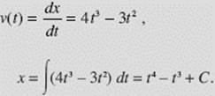
Since x(0) = 0⁴ − 0³ + C = 3, we see that C = 3, and that the position function is x(t) = t⁴ − t³ + 3. When t = 2, we see that

x(2) = 2⁴ − 2³ + 3 = 16 − 8 + 3 = 11.

EXAMPLE 51

Suppose that a(t), the acceleration of a particle at time t, is given by a(t) = 4t − 3, that v(1) = 6, and that f (2) = 5, where f (t) is the position function.

(a) Find v(t) and f (t).

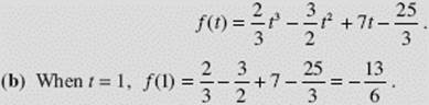
(b) Find the position of the particle when t = 1.

SOLUTIONS:

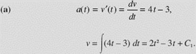
Using v(1) = 6, we get 6 = 2(1)² − 3(1) + C₁, and C₁ = 7, from which it follows that v(t) = 2t² − 3t + 7. Since

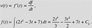
Using f (2) = 5, we get + 14 + C₂, so Thus,

For more examples of motion along a line, see Chapter 8, Further Applications of Integration, and Chapter 9, Differential Equations.

Chapter Summary

In this chapter, we have reviewed basic skills for finding indefinite integrals. We’ve looked at the antiderivative formulas for all of the basic functions and reviewed techniques for finding antiderivatives of other functions.

We’ve also reviewed the more advanced techniques of integration by partial fractions and integration by parts, both topics only for the BC Calculus course.