Calculus AB and Calculus BC

CHAPTER 6 Definite Integrals

E. APPROXIMATIONS OF THE DEFINITE INTEGRAL; RIEMANN SUMS

It is always possible to approximate the value of a definite integral, even when an integrand cannot be expressed in terms of elementary functions. If f is nonnegative on [a, b], we interpret dx as the area bounded above by y = f (x), below by the x-axis, and vertically by the lines x = a andx = b. The value of the definite integral is then approximated by dividing the area into n strips, approximating the area of each strip by a rectangle or other geometric figure, then summing these approximations. We often divide the interval from a to b into n strips of equal width, but any strips will work.

E1. Using Rectangles.

We may approximate by any of the following sums, where Δx represents the

subinterval widths:

(1) Left sum: f (x₀) Δx₁ + f (x₁) Δx₂ + … + f (x_{n − 1}) Δx_n, using the value of f at the left endpoint of each subinterval.

(2) Right sum: f (x₁) Δx₁ + f (x₂) Δx₂ + … + f (x_n) Δx_n, using the value of f at the right end of each subinterval.

(3) Midpoint sum: using the value of f at the midpoint of each subinterval.

These approximations are illustrated in Figures N6–4 and N6–5, which accompany Example 24.

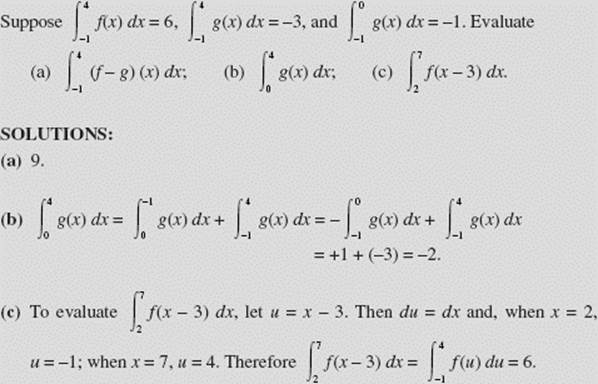
EXAMPLE 24

Approximate by using four subintervals of equal width and calculating:

(a) the left sum,

(b) the right sum,

(c) the midpoint sum, and (d) the integral.

SOLUTIONS: Here

(a) For a left sum we use the left-hand altitudes at The approximating sum is

The dashed lines in Figure N6–4 show the inscribed rectangles used.

(b) For the right sum we use right-hand altitudes at and 2. The approximating sum is

This sum uses the circumscribed rectangles shown in Figure N6–4.

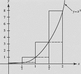
FIGURE N6–4

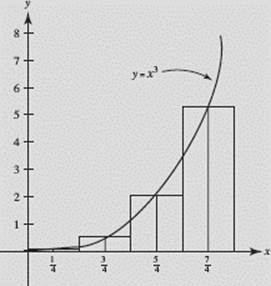
FIGURE N6–5

(c) The midpoint sum uses the heights at the midpoints of the subintervals, as shown in Figure N6–5. The approximating sum is

(d) Since the exact value of or 4, the midpoint sum is the best of the three approximations. This is usually the case.

We will denote the three Riemann sums, with n subintervals, by L(n), R(n), and M(n). (These sums are also sometimes called “rules.”)

E2. Using Trapezoids.

We now find the areas of the strips in Figure N6–6 by using trapezoids. We denote the bases of the trapezoids by y₀, y₁, y₂, …, y_n and the heights by Δx = h₁, h₂, …, h_n.

FIGURE N6–6

The following sum approximates the area between f and the x-axis from a to b:

If all subintervals are of equal width, h, we can remove the common factor

Trapezoid Rule

Using T(n) to denote the approximating sum with n equal subintervals, we have the Trapezoid Rule:

EXAMPLE 25

Use T(4) to approximate

SOLUTION: From Example Then,

This is better than either L(4) or R(4), but M(4) is the best approximation here.

EXAMPLE 26

A function f passes through the five points shown. Estimate the area using (a) a left rectangular approximation and

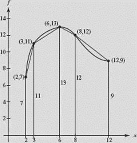
(b) a trapezoidal approximation.

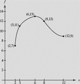
SOLUTION: Note that the subinterval widths are not equal.

(a) In each subinterval, we sketch the rectangle with height determined by the point on f at the left end-point. Our estimate is the sum of the areas of these rectangles:

A ≈ 1(7) + 3(11) + 2(13) + 4(12) ≈ 114

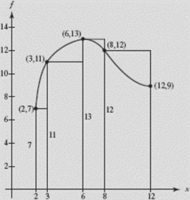
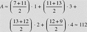
(b) In each subinterval, we sketch trapezoids by drawing segments connecting the points on f. Our estimate is the sum of the areas of these trapezoids:

Comparing Approximating Sums

If f is an increasing function on [a,b], then while if f is decreasing, then

From Figure N6–7 we infer that the area of a trapezoid is less than the true area if the graph of f is concave down, but is more than the true area if the graph of f is concave up.

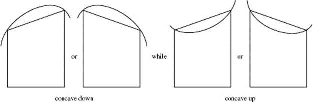
FIGURE N6–7

Figure N6–8 is helpful in showing how the area of a midpoint rectangle compares with that of a trapezoid and with the true area. Our graph here is concave down. If M is the midpoint of AB, then the midpoint rectangle is AM₁ M₂ B. We’ve drawn T₁ T₂ tangent to the curve at T (where the midpoint ordinate intersects the curve). Since the shaded triangles have equal areas, we see that area AM₁ M₂ B = area AT₁ T₂ B.^† But area AT₁ T₂ B clearly exceeds the true area, as does the area of the midpoint rectangle. This fact justifies the right half of the inequality below; Figure N6–7verifies the left half.

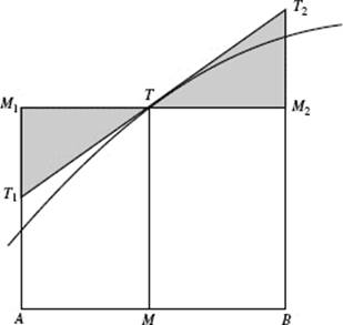
FIGURE N6–8

Generalizing to n subintervals, we conclude:

If the graph of f is concave down, then

If the graph of f is concave up, then

EXAMPLE 27

Write an inequality including L(n), R(n), M(n), T(n), and for the graph of f shown in Figure N6–9.

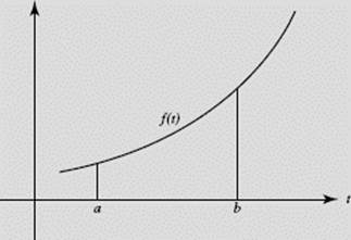
FIGURE N6–9

^† Note that the trapezoid AT₁ T₂ B is different from the trapezoids in Figure N6–7, which are like the ones we use in applying the trapezoid rule.

SOLUTION: Since f increases on [a,b] and is concave up, the inequality is

Graphing a Function from Its Derivative; Another Look

EXAMPLE 28

Figure N6–10 is the graph of function f ′(x); it consists of two line segments and a semicircle. If f (0) = 1, sketch the graph of f (x). Identify any critical or inflection points of f and give their coordinates.

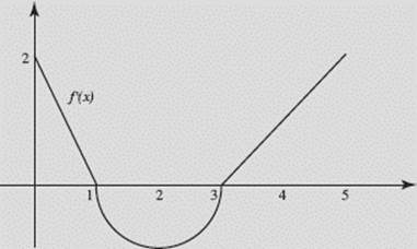
FIGURE N6–10

SOLUTION: We know that if f ′ > 0 on an interval then f increases on the interval, while if f ′ < 0 then f decreases; also, if f ′ is increasing on an interval then the graph of f is concave up on the interval, while if f ′ is decreasing then the graph of f is concave down. These statements lead to the following conclusions:

Additionally, Since f ′(1) = f ′(3) = 0, f has critical points at x = 1 and x = 3. As x passes through 1, the sign of f ′ changes from positive to negative; as x passes through 3, the sign of f ′ changes from negative to positive. Therefore f (1) is a local maximum and f (3) a local minimum. Since fchanges from concave down to concave up at x = 2, there is an inflection point on the graph of f there.

These conclusions enable us to get the general shape of the curve, as displayed in Figure N6–11a.

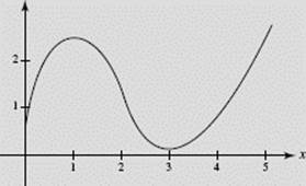
FIGURE N6–11a

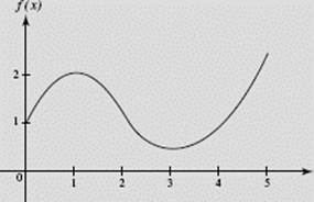
FIGURE N6–11b

All that remains is to evaluate f (x) at x = 1, 2, and 3. We use the Fundamental Theorem of Calculus to accomplish this, finding f also at x = 4 and 5 for completeness.

We are given that f (0) = 1. Then

where the integral yields the area of the triangle with height 2 and base 1;

where the integral gives the area of a quadrant of a circle of radius 1 (this integral is negative!);

where the integral is the area of the triangle with height 1 and base 1;

So the function f (x) has a local maximum at (1,2), a point of inflection at (2,1.2), and a local minimum at (3,0.4) where we have rounded to one decimal place when necessary.

In Figure N6–11b, the graph of f is shown again, but now it incorporates the information just obtained using the FTC.

EXAMPLE 29

Readings from a car’s speedometer at 10-minute intervals during a 1-hour period are given in the table; t = time in minutes, v = speed in miles per hour:

(a) Draw a graph that could represent the car’s speed during the hour.

(b) Approximate the distance traveled, using L(6), R(6), and T(6).

(c) Draw a graph that could represent the distance traveled during the hour.

SOLUTIONS:

(a) Any number of curves will do. The graph has only to pass through the points given in the table of speeds, as does the graph in Figure N6–12a.

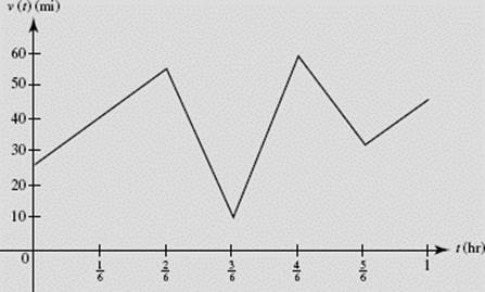
FIGURE N6–12a

(b) L(6) = (26 + 40 + 55 + 10 + 60 + 32) ·

R(6) = (40 + 55 + 10 + 60 + 32 + 45) ·

(26 + 2 · 40 + 2 · 55 + 2 · 10 + 2 · 60 + 2 · 32 + 45) =

(c) To calculate the distance traveled during the hour, we use the methods demonstrated in Example 28. (We know that, since v(t) > 0, is the distance covered from time a to time b, where v(t) is the speed or velocity). Thus,

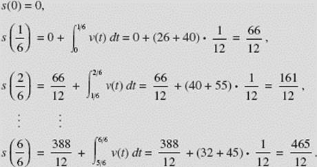
It is left to the student to complete the missing steps above and to verify the distances in the following table (t = time in minutes, s = distance in miles):

Figure N6–12b is one possible graph for the distance covered during the hour.

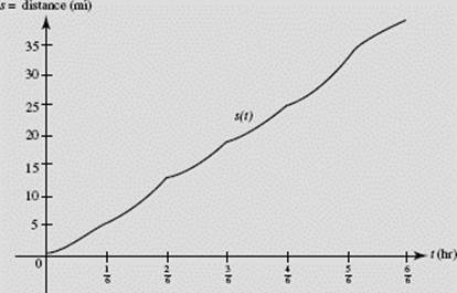
FIGURE N6–12b

EXAMPLE 30

The graph of f (t) is given in Figure N6–13. fill in the values for F(x) in the table:

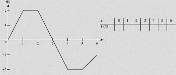
FIGURE N6–13

SOLUTION: We evaluate F(x) by finding areas of appropriate regions.

Here is the completed table:

EXAMPLE 31

The graph of the function f(t) is shown in Figure N6–14.

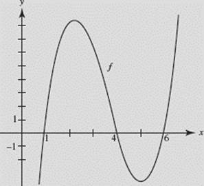
FIGURE N6–14

Let Decide whether each statement is true or false; justify your

answers:

(i) If 4 < x < 6, F(x) > 0.

(ii) If 4 < x < 5, F ′(x) > 0.

(iii) F ″(6) < 0.

SOLUTIONS:

(i) is true. We know that, if a function g is positive on (a, b), then whereas if g is negative on (a, b), then However, the area above the x-axis between x = 1 and x = 4 is greater than that below the axis between 4 and 6. Since

it follows that F(x) > 0 if 4 < x < 6.

(ii) is false. Since F ′(x) = f (x) and f (x) < 0 if 4 < x < 5, then F ′(x) < 0.

(iii) is false. Since F ′(x) = f (x), F ″ (x) = f ′(x). At x = 6, f ′(x) > 0 (because f is increasing). Therefore, F ″(6) > 0.

EXAMPLE 32

Graphs of functions f (x), g(x), and h(x) are given in Figures N6–15a, N6–15b, and N6–15c. Consider the following statements:

(I) f (x) = g ′(x) (II) h(x) = f ′(x) (III)

Which of these statements is (are) true?

(A) I only

(B) II only

(C) III only

(D) all three

(E) none of them

SOLUTION:

The correct answer is D.

I is true since, for example, f (x) = 0 for the critical values of g: f is positive where g increases, negative where g decreases, and so on.

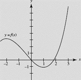
FIGURE N6–15a

II is true for similar reasons.

III is also true. Verify that the value of the integral g(x) increases on the interval −2.5 < x < 0 (where f > 0), decreases between the zeros of f (where f < 0), then increases again when f becomes positive.

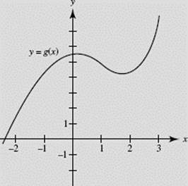
FIGURE N6–15b

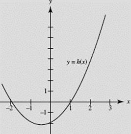
FIGURE N6–15c

EXAMPLE 33

Assume the world use of copper has been increasing at a rate given by f (t) = 1.5e^0.015t, where t is measured in years, with t = 0 the beginning of 2000, and f (t) is measured in millions of tons per year.

(a) What definite integral gives the total amount of copper that was used for the 5-year period from t = 0 to the beginning of the year 2005?

(b) Write out the terms in the left sum L(5) for the integral in (a). What do the individual terms of L(5) mean in terms of the world use of copper?

(c) How good an approximation is L(5) for the definite integral in (a)?

SOLUTIONS:

(a)

(b) L(5) = 15e^{0.015 · 0} + 15e^{0.015 · 1} + 15e^{0.015 · 2} + 15e^{0.015 · 3} + 15e^{0.015 · 4}. The five terms on the right represent the world’s use of copper for the 5 years from 2000 until 2005.

(c) The answer to (a), using our calculator, is 77.884 million tons. L(5) = 77.301 million tons, so L(5) underestimates the projected world use of copper during the 5-year period by approximately 583,000 tons.

Example 32 is an excellent instance of the FTC: if f = F ′ then gives the total change in F as x varies from a to b.

EXAMPLE 34