Calculus AB and Calculus BC

CHAPTER 1 Functions

F. PARAMETRICALLY DEFINED FUNCTIONS

BC ONLY

If the x- and y-coordinates of a point on a graph are given as functions f and g of a third variable, say t, then

x = f (t), y = g(t)

are called parametric equations and t is called the parameter. When t represents time, as it often does, then we can view the curve as that followed by a moving particle as the time varies.

Examples 12–18 are BC ONLY.

EXAMPLE 12

Find the Cartesian equation of, and sketch, the curve defined by the parametric equations

x = 4 sin t, y = 5 cos t (0 t 2π).

SOLUTION: We can eliminate the parameter t as follows:

Since sin² t + cos² t = 1, we have

The curve is the ellipse shown in Figure N1–9.

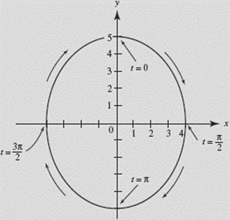
FIGURE N1–9

Note that, as t increases from 0 to 2π, a particle moving in accordance with the given parametric equations starts at point (0, 5) (when t = 0) and travels in a clockwise direction along the ellipse, returning to (0, 5) when t = 2π.

EXAMPLE 13

Given the pair of parametric equations,

x = 1 − t, y = (t 0),

write an equation of the curve in terms of x and y, and sketch the graph.

SOLUTION: We can eliminate t by squaring the second equation and substituting for t in the first; then we have

y² = t and x = 1 − y².

We see the graph of the equation x = 1 − y² on the left in Figure N1–10. At the right we see only the upper part of this graph, the part defined by the parametric equations for which t and y are both restricted to nonnegative numbers.

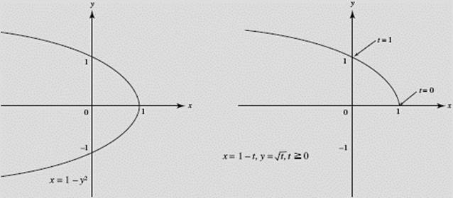
FIGURE N1–10

The function defined by the parametric equations here is y = F(x) = whose graph is at the right above; its domain is x 1 and its range is the set of nonnegative reals.

EXAMPLE 14

A satellite is in orbit around a planet that is orbiting around a star. The satellite makes 12 orbits each year. Graph its path given by the parametric equations

x = 4 cos t + cos 12t,

y = 4 sin t + sin 12t.

SOLUTION: Shown below is the graph of the satellite’s path using the calculator’s parametric mode for 0 ≤ t ≤ 2π.

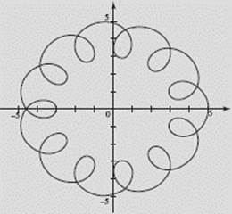
FIGURE N1–11

EXAMPLE 15

Graph x = y² − 6y + 8.

SOLUTION: We encounter a difficulty here. The calculator is constructed to graph y as a function of x: it accomplishes this by scanning horizontally across the window and plotting points in varying vertical positions. Ideally, we want the calculator to scan down the window and plot points at appropriate horizontal positions. But it won’t do that.

One alternative is to interchange variables, entering x as Y₁ and y as X, thus entering Y₁, = X² − 6X + 8. But then, during all subsequent processing we must remember that we have made this interchange.

Less risky and more satisfying is to switch to parametric mode: Enter x = t² − 6t + 8 and y = t. Then graph these equations in [−10,10] × [−10,10], for t in [−10,10], See Figure N1–12.

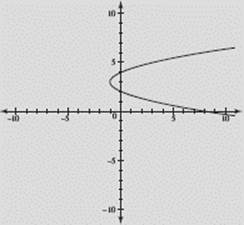
FIGURE N1–12

EXAMPLE 16

Let f (x) = x³ + x; graph f ⁻¹(x).

SOLUTION: Recalling that f ⁻¹ interchanges x and y, we use parametric mode to graph

f: x = t, y = t³ + t
and f ⁻¹: x = t³ + t, y = t.

Figure N1–13 shows both f (x) and f ⁻¹(x).

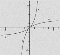
FIGURE N1–13

Parametric equations give rise to vector functions, which will be discussed in connection with motion along a curve in Chapter 4.