Burn Math Class: And Reinvent Mathematics for Yourself (2016)

2. The Infinite Power of the Infinite Magnifying Glass

2.4. Hunting Extremes in the Dark

Extremes are interesting. Watching an Olympic gold medalist sprint or swim or throw a javelin is generally more captivating than watching a randomly chosen person from your neighborhood doing the same thing. We enjoy watching the superlative performances of people who are the best at some particular activity. On the other extreme, the worst performances in any given category have a similar power to draw our attention. The principle that extremes are interesting also tends to be true in the world of mathematics. It may come in handy to be able to locate those extremes — places where a given quantity is largest or smallest, highest or lowest, best or worst — and to do so simply by manipulating symbols, since we won’t always be able to visualize the objects we’re studying.

Without even realizing it, we gained a surprisingly powerful ability when we invented the concept of the derivative: the ability to hunt down the locations where a machine achieves its extremes, even if we can’t even begin to picture what the machine looks like! Here’s the idea.

Since a machine’s derivative tells us the slope of the machine at that point, we can make use of the following convenient fact: all flat points of a machine are places where that machine’s derivative is zero. As such, we can find the flat points of a machine m by forcing its derivative to be zero

and then trying to figure out which numbers x make that sentence true. If we can figure that out, then we will have found the flat points of the machine. Then we just have to check a small number of cases to see where the extremes are. Importantly, we can do this even if we can’t visualize what the machine looks like.

Let’s look at a few simple examples of this. Back in Figure 2.3, we drew a picture of the Times Self Machine m(x) ≡ x². It’s apparent from the picture that this machine has no maximum (it keeps getting bigger as x gets further from zero, in either direction), but it clearly has a minimum at x = 0. Now, even if we couldn’t picture this machine, we could still coax the mathematics into telling us where the minimum is. Since m(x) ≡ x², we already know that m′(x) = 2x. Now we can just write down the sentence “this machine’s derivative at x is zero” in symbolic form, like this:

I used because the sentence 2x = 0 isn’t always true, so the helps us remember that it’s something we’re forcing to be true (i.e., something we’re insisting on), in order to see which particular x’s actually make the sentence true. Which x’s are those? Fortunately, it’s not too hard to see that 2x = 0 only when x = 0, which tells us that the machine m(x) ≡ x² has one and only one flat point, and it lives at x = 0. We knew this in advance (from the pictures we drew earlier), but it’s always nice to test our new ideas on familiar cases to make sure they give what we expect. That’s how we can check what we’ve done, in our own private universe, without requiring the help of a textbook or an authority figure.

Similarly, what if we looked at the machine f(x) ≡ (x−3)²? In a sense, this is just like the previous example. Anything that looks like (stuff)² is going to be positive unless stuff = 0, so we might expect that this machine would have one and only one flat point, at x = 3, and that this point would be a minimum, just like last time. Now, that’s all correct, but suppose we were handed this same machine in a form that made its similarity to (stuff)² less clear, namely:

f(x) ≡ x² − 6x + 9

This is exactly the same machine as f(x) ≡ (x − 3)², but it’s less clear from looking at the above equation that it will have one and only one flat point at x = 3. Nevertheless, we can get the mathematics to tell us this fact using the same idea we used above — compute the derivative, and force it to be equal to zero:

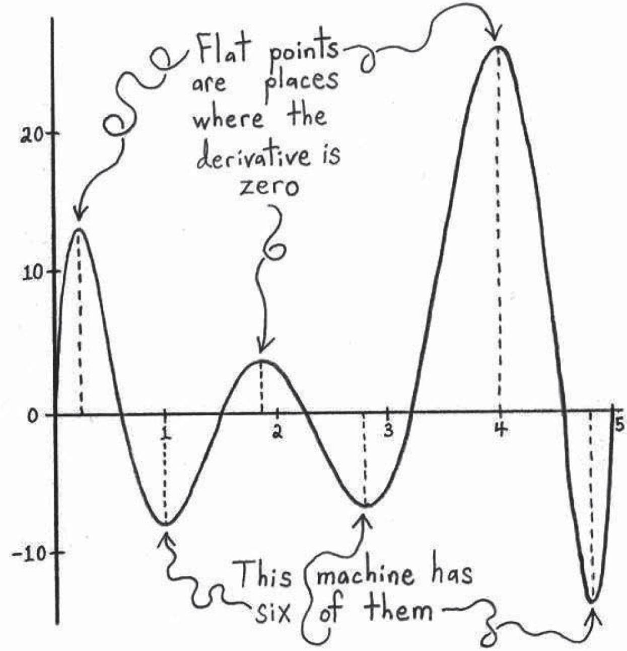
Figure 2.5: This machine has six flat points. If we describe them by their horizontal coordinates, then the flat points occur when x is 0.25-ish, 1, 1.8-ish, 2.7-ish, 4, and 4.8-ish. Not all of the flat points are extremes, but both of the extremes are flat points. That is, the maximum of this machine in the region pictured is at the flat point x = 4, while the minimum of this machine in the region pictured is at the flat point x ≈ 4.8.

Now, the sentence 2x − 6 = 0 is saying the same thing as the sentence 2x = 6, which is saying the same thing as the sentence x = 3. So just as we expected, we were able to figure out that this machine has one and only one flat point, and its location is at x = 3. And the fact that we got the same result in two different ways provides further evidence that our ideas make sense.

It is important to notice that this idea will not always spit out the extremes (i.e., the maximum spots and minimum spots) of a given machine. However, this is not because of a failure of the mathematics, but rather because of a few obvious facts we overlooked. To get the idea, let’s look at a few examples. Suppose we wanted to find the maximum of the machine g(x) ≡ 2x, and we proceed using the ideas above. We find its derivative and force it to be equal to zero, which gives

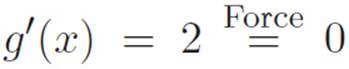
The “force the derivative to be zero” method has just spat out the ridiculous sentence 2 = 0. Does this mean that 2 is really equal to 0? Hopefully not! Does it mean that the “force the derivative to be zero” method of finding extreme points has broken down? Not really. The graph of the machineg(x) ≡ 2x is a tilted line, and straight lines have no flat points, unless the whole line is horizontal (I drew a picture of this in Figure 2.6, but it’s hardly necessary). This failure is not a flaw of the “force the derivative to be zero” method. Rather, by spitting out something impossible like 2 = 0, the mathematics is simply telling us that we assumed something impossible. Not a mystery.

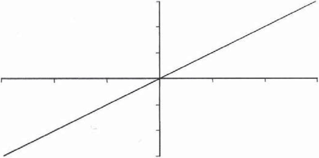
Figure 2.6: This machine has no flat (i.e., horizontal) points. When we try to force the mathematics to tell us where they are, it tells us that 2 = 0. Don’t worry, it’s just messing with us. This is how the mathematics typically lets us know that one of our assumptions was wrong.

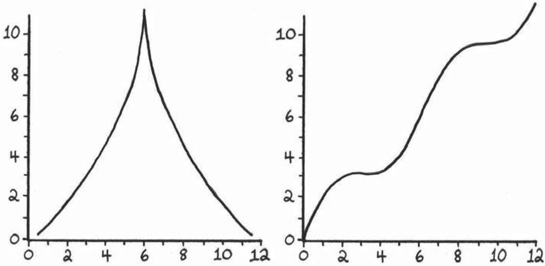
Figure 2.7: Above, we discussed the strategy of finding the highest and lowest parts of a machine by figuring out where its derivative is zero. In a perfect world, that strategy would always work, but there are some obnoxious situations where it doesn’t. I should at least mention them briefly, though we won’t run into them after this. The machine on the left has a maximum, but it occurs at an infinitely pointy place, where the derivative won’t spit out zero, so the “force the derivative to be zero” method will miss it. Fortunately, these infinitely pointy machines don’t show up unless we ask them to, so we won’t have to deal with finding the extremes of any of them in this book. The machine on the right has two flat points in the region pictured, but neither of them is an extreme point (i.e., neither is a maximum or a minimum). As such, the “force the derivative to be zero” method would spit out the locations of these more boring flat points, which are located somewhere near x ≈ 3 and at x ≈ 9 (the squiggly equals sign means “roughly”).

Although unfortunate examples like those in Figure 2.7 won’t be showing up much in the book, a brief mention of them is important if you want to understand the odd way that mathematicians write. Mathematicians tend to be somewhat obsessed with “counterexamples” — rare, bizarre exceptions to simple rules — and this obsession makes their theorems much harder to read. For example, in describing the “derivative equals zero” method, a mathematician might say: “Let f: (a, b) → be a function and suppose that x₀ ∈ (a, b) is a local extremum of f, where f is differentiable atx₀. Then f′(x₀) = 0.” That probably sounds like gibberish, but what they’re really trying to say is pretty simple. The translation would be something like: “Picture the highest (or lowest) point on the graph of some machine. The machine has to be flat there. Oops, I mean, unless it’s infinitely pointy, like on the left side of Figure 2.7. But that doesn’t happen very often.” The exception on the right side of Figure 2.7 shows up in the above theorem too, but it’s more hidden. It’s the reason why the gibberish is saying:

“If we’re at a max or min, then the derivative is zero”

rather than

“If the derivative is zero, then we’re at a max or min”

The second sentence would be true if it weren’t for flat points like the ones on the right side of Figure 2.7 (where the derivative is zero, but we’re not at a max or min). If such unfortunate examples didn’t exist, then they could say the second sentence instead of the first, and that would be much more convenient, since the point of all this “derivative equals zero” business is usually to figure out where those max and min points are.

Okay! So, even though there are exceptions, we will continue to run into this idea throughout the book: the extremes of a given machine can usually be found by figuring out where the derivative of that machine is zero. As we generalize the notion of the derivative to more exotic types of machines, the way we will have to state this idea will change slightly, but the central idea will remain the same. For machines that eat one number and spit out one number, for machines that eat two numbers and spit out one number, for machines that eat N numbers and spit out one number, and finally for machines that eat infinitely many numbers and spit out one number, the basic principle that “extremes are usually places where the derivative equals zero” will continue to apply no matter how far we go, and no matter how strange our mathematical universe becomes.