Burn Math Class: And Reinvent Mathematics for Yourself (2016)

6. Two in One

6.1. Two is One

6.1.1Another Abbreviation Becomes an Idea

In the previous interlude, we discussed the problem of finding the areas of curvy things. We eventually gave up, but we had one minor insight. When we zoom in on the graph of a machine at any point x, the tiny sliver of area under that point can be thought of as an infinitely thin rectangle with height m(x) and width dx. So the area hiding under a machine’s graph at any point x should just be m(x)dx. But hypothetically, if we could somehow add up all the areas of those infinitely thin rectangles under every point x (say, every point between x = a and x = b), then we should get the total (possibly curvy) area under the graph of m.

We have no idea how to actually do this. However, we wrote down a great abbreviation to summarize the idea: 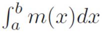. This abbreviation reflects the fact that we can think of a curvy area as the sum (hence the S-like ∫ thing) of an infinite number of infinitely thin rectangles (hence them(x)dx). But this was just an abbreviation for the (unknown) answer. It didn’t tell us how to actually calculate curvy areas.

Anyone would be likely to get stuck here for awhile. However, that dx in our new abbreviation is suggestive. We’ve seen that symbol before, sitting on the bottom of a derivative. Maybe using our old derivative idea will help us to understand our new ∫ idea.

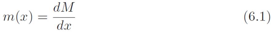
Derivatives are machines, too. For example, something like f(s) ≡ s² has the derivative f′(s) ≡ 2s, and that 2s is a machine just as much as x² was. So, suppose the m(x) inside our funny ∫ symbol is really the derivative of some other machine M(x). That would let us write

If we think of m this way, then we can pull the following tricky move to rewrite our abbreviation for the (unknown) curvy area:

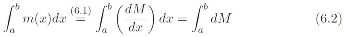
The symbol dM was just our abbreviation for M(x + dx) − M(x), a tiny change in height between two points that are infinitely close together. So the meaning of the symbol is this: walk from x = a to x = b, and add up all the tiny changes in height you experience along the way.

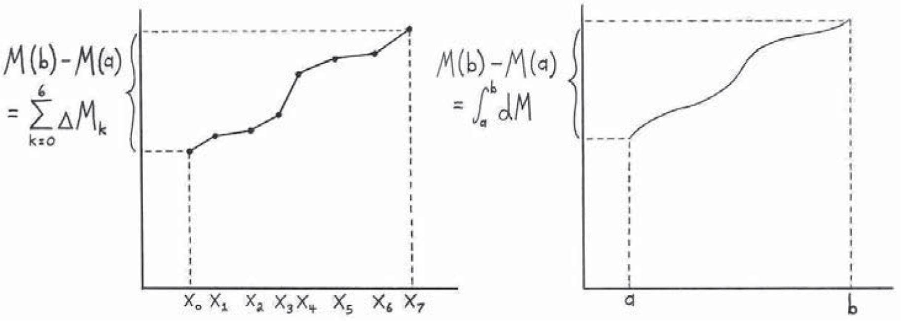
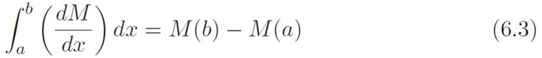
Figure 6.1: Visualizing the reason why 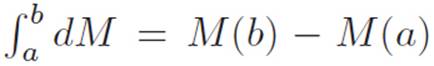. The first picture demonstrates the idea for machines whose graphs are made up of a finite number of straight lines. The total height change between a and b can be thought of in two ways. On the one hand, the height change is M(end) − M(beginning) (that is, M(b) − M(a) for the picture on the right, or M(x₇) − M(x₀) for the picture on the left). On the other hand, the total height change is just the sum of all the tiny height changes experienced in each “step” as we walk along the machine’s graph. Each of these tiny changes is of the form ΔM_k ≡ M(x_k+1) − M(x_k). In the truly curvy case on the right, the same idea holds, but now there are an infinite number of infinitely small steps, each of which gives us an infinitely small change in height dM. The sum of all these infinitely small changes in height (i.e., ) is just the total change in height (i.e., M(b) − M(a)).

Now, since the symbol stands for “whatever we would get if we could somehow add up all the tiny changes in height between a and b,” then it must just refer to the total change in height between a and b, which is to say M(end) − M(beginning), or equivalently, M(b) − M(a). If this isn’t clear, then the pictures in Figure 6.1 might help. Alright, using this fact, we can extend the above equation by one step, and summarize the gist of it by writing

And now we’re stuck aga. . . wait a second. Are we done?

6.1.2The Fundamental Hammer of Calculus

There’s no way this is correct — it’s too simple. It says that this new ∫ symbol we wrote down, just as a meaningless abbreviation for the area under a curve, turns out to be sort of the opposite of the derivative idea we invented earlier. That is, starting with M, then finding its derivative, then applying the “area under me” operation to that, we get something just involving M; something that involves neither derivatives nor the “area under me” operation. Equation 6.3 is a sentence that relates the two main calculus ideas we’ve invented so far: namely, computing curvy steepness (differentiation) and curvy areas (“integration,” in textbook jargon). Because it ties our two main ideas together, let’s call it the fundamental hammer of calculus. Now we can rephrase equation 6.3 by writing this:

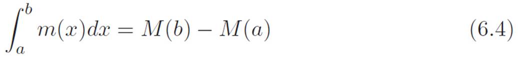
where M is any machine whose derivative is m. So this says that if we want to find the area under some curvy thing m between two points x = a and x = b, then all we have to do is think of an “anti-derivative” of m, that is, a machine M whose derivative is the machine m that we started with. If we can somehow do that, then the area under m is just M(b) − M(a). So whenever we can think of an anti-derivative of a given machine, the seemingly impossible problem of computing its (possibly curvy) area is simple! Armed with an anti-derivative of m, we can find curvy areas using nothing but subtraction.

As always, it’s worth checking our idea in a few simple cases where we already know what to expect. If it gives us the wrong answers in those simple cases, then our new idea is broken and we have to start over. However, if the crazy argument above is correct, then that would mean we’d get two ideas for the price of one; the ∫ idea (computing curvy areas) would just be the derivative idea (computing curvy slopes) in reverse. Let’s do some field-testing on this new idea of ours.