Calculus II For Dummies, 2nd Edition (2012)
Part III. Intermediate Integration Topics
In this part . . .
With the basics of calculating integrals under your belt, the focus becomes using integration as a problem-solving tool. You discover how to solve more complex area problems and how to find the surface area and volume of solids.
Chapter 9. Forging into New Areas: Solving Area Problems
In This Chapter
![]() Evaluating improper integrals
Evaluating improper integrals
![]() Solving area problems with more than one function
Solving area problems with more than one function
![]() Measuring the area between functions
Measuring the area between functions
![]() Finding unsigned areas
Finding unsigned areas
![]() Understanding the Mean Value Theorem and calculating average value
Understanding the Mean Value Theorem and calculating average value
![]() Figuring out arc length
Figuring out arc length
With your toolbox now packed with the hows of calculating integrals, this chapter (and Chapter 10) introduces you to some of the whys of calculating them.
I start with a simple rule for expressing an area as two separate definite integrals. Then I focus on improper integrals, which are integrals that are either horizontally or vertically infinite. Next, I give you a variety of practical strategies for measuring areas that are bounded by more than one function. I look at measuring areas between functions, and I also get you clear on the distinction between signed area and unsigned area.
After that, I introduce you to the Mean Value Theorem for Integrals, which provides the theoretical basis for calculating average value. Finally, I show you a formula for calculating arc length, which is the exact length between two points along a function.
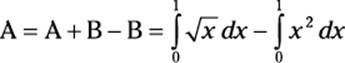
Breaking Us in Two
Here’s a simple but handy rule that looks complicated but is really very easy:
![]()
This rule just says that you can split an area into two pieces and then add up the pieces to get the area that you started with.
For example, the entire shaded area in Figure 9-1 is represented by the following integral, which you can evaluate easily:
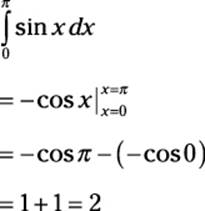
Figure 9-1:Splitting the area ![]() into two smaller pieces.
into two smaller pieces.
Drawing a vertical line at ![]() and splitting this area into two separate regions results in two separate integrals:
and splitting this area into two separate regions results in two separate integrals:
It should come as no great shock that the sum of these two smaller regions equals the entire area:
Although this idea is ridiculously simple, splitting an integral into two or more integrals becomes a powerful tool for solving a variety of the area problems in this chapter.
Improper Integrals
Improper integrals come in two varieties — horizontally infinite and vertically infinite:
![]() A horizontally infinite improper integral contains either ∞ or –∞ (or both) as a limit of integration. See the next section, “Getting horizontal,” for examples of this type of integral.
A horizontally infinite improper integral contains either ∞ or –∞ (or both) as a limit of integration. See the next section, “Getting horizontal,” for examples of this type of integral.
![]() A vertically infinite improper integral contains at least one vertical asymptote. I discuss this further in the later section “Going vertical.”
A vertically infinite improper integral contains at least one vertical asymptote. I discuss this further in the later section “Going vertical.”
Improper integrals become useful for solving a variety of problems in Chapter 10. They’re also useful for getting a handle on infinite series in Chapter 11. Evaluating an improper integral is a three-step process:
1. Express the improper integral as the limit of an integral.
2. Evaluate the integral by whatever method works.
3. Evaluate the limit.
In this section, I show you, step by step, how to evaluate both types of improper integrals.
Getting horizontal
The first type of improper integral occurs when a definite integral has a limit of integration that’s either ∞ or –∞. This type of improper integral is easy to spot because infinity is right there in the integral itself. You can’t miss it.
For example, suppose that you want to evaluate the following improper integral:
![]()
Here’s how you do it, step by step:
1. Express the improper integral as the limit of an integral.
When the upper limit of integration is ∞, use this equation:
![]()
So here’s what you do:
![]()
2. Evaluate the integral:
3. Evaluate the limit:
![]()
Before moving on, reflect for one moment that the area under an infinitely long curve is actually finite. Ah, the magic and power of calculus!
Similarly, suppose that you want to evaluate the following:
![]()
Here’s how you do it:
1. Express the integral as the limit of an integral.
When the lower limit of integration is –∞, use this equation:
![]()
So here’s what you write:
![]()
2. Evaluate the integral:
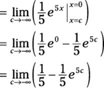
3. Evaluate the limit — in this case, as c approaches –∞, the first term is unaffected and the second term approaches 0:
![]()
Again, calculus tells you that, in this case, the area under an infinitely long curve is finite.
Of course, sometimes the area under an infinitely long curve is infinite. In these cases, the improper integral can’t be evaluated because the limit does not exist (DNE). Here’s a quick example that illustrates this situation:
![]()
It may not be obvious that this improper integral represents an infinitely large area. After all, the value of the function approaches 0 as x increases. But watch how this evaluation plays out:
1. Express the improper integral as the limit of an integral:
![]()
2. Evaluate the integral:
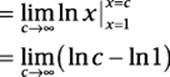
At this point, you can see that the limit explodes to infinity, so it doesn’t exist. Therefore, the improper integral can’t be evaluated, because the area that it represents is infinite.
Going vertical
Vertically infinite improper integrals are harder to recognize than those that are horizontally infinite. An integral of this type contains at least one vertical asymptote in the area that you’re measuring. (A vertical asymptote is a value of x where f(x) equals either ∞ or –∞. See Chapter 2 for more on asymptotes.) The asymptote may be a limit of integration or it may fall someplace between the two limits of integration.
 Don’t try to slide by and evaluate improper integrals as proper integrals. In most cases, you’ll get the wrong answer!
In this section, I show you how to handle both cases of vertically infinite improper integrals.
Handling asymptotic limits of integration
Suppose that you want to evaluate the following integral:

At first glance, you may be tempted to evaluate this as a proper integral. But this function has an asymptote at x = 0. The presence of an asymptote at one of the limits of integration forces you to evaluate this one as an improper integral:
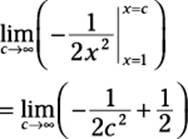
1. Express the integral as the limit of an integral:
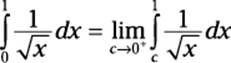
Notice that in this limit, c approaches 0 from the right — that is, from the positive side — because this is the direction of approach from inside the limits of integration. (That’s what the little plus sign (+) in the limit means.)
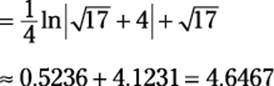
2. Evaluate the integral:
This integral is easily evaluated as ![]() , using the Power Rule as I show you in Chapter 4, so I spare you the details here:
, using the Power Rule as I show you in Chapter 4, so I spare you the details here:
![]()
3. Evaluate the limit:
![]()
At this point, direct substitution provides you with your final answer:
= 2
Piecing together discontinuous integrands
In Chapter 3, I discuss the link between integrability and continuity: If a function is continuous on an interval, it’s also integrable on that interval. (Flip to Chapter 3 for a refresher on this concept.)
Some integrals that are vertically infinite have asymptotes not at the edges but someplace in the middle. The result is a discontinuous integrand — that is, a function with a discontinuity on the interval that you’re trying to integrate.
Discontinuous integrands are the trickiest improper integrals to spot — you really need to know how the graph of the function that you’re integrating behaves. (See Chapter 2 to see graphs of the elementary functions.)
To evaluate an improper integral of this type, separate it at each asymptote into two or more integrals, as I demonstrate earlier in this chapter in “Breaking Us in Two.” Then evaluate each of the resulting integrals as an improper integral, as I show you in the previous section.
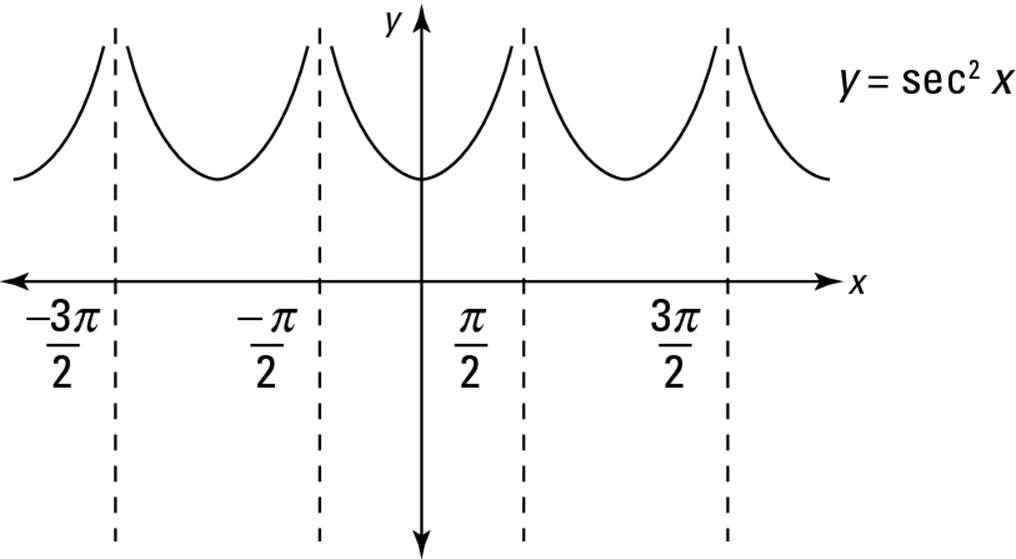
For example, suppose that you want to evaluate the following integral:
![]()
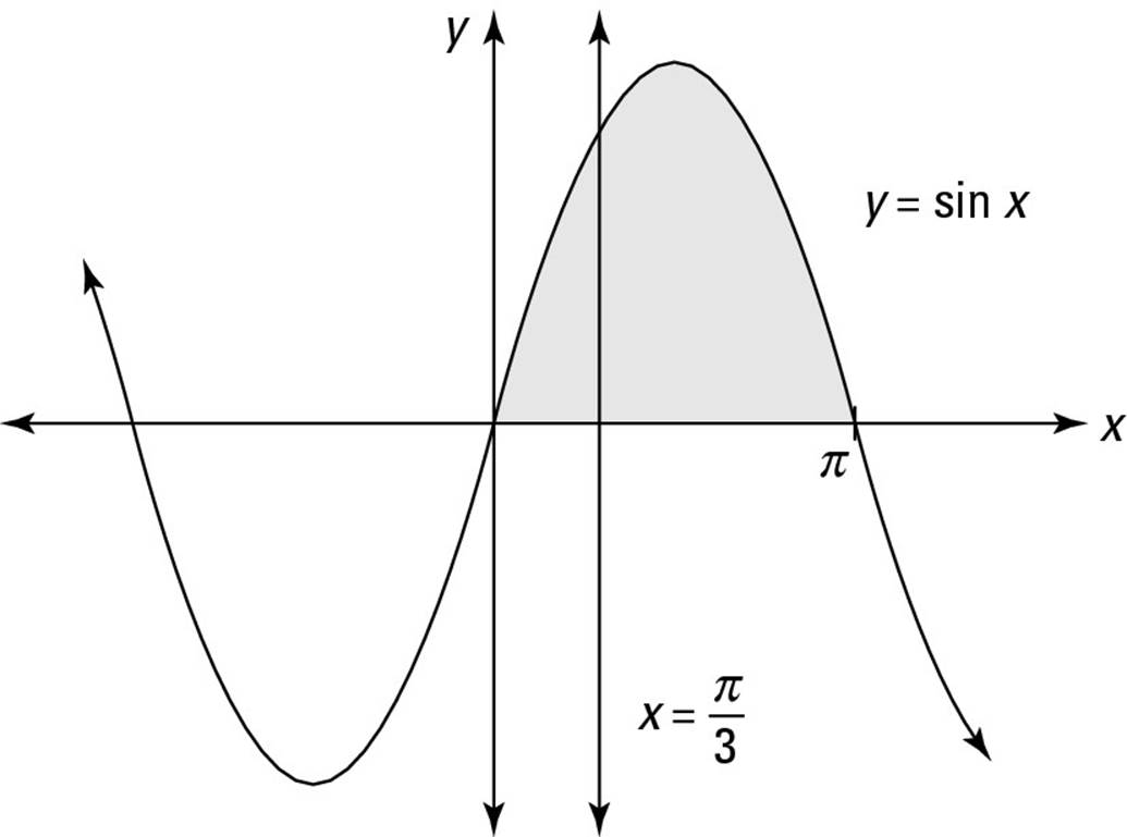
Because the graph of sec x contains an asymptote at ![]() (see Chapter 2 for a view of this graph), the graph of sec2 x has an asymptote in the same place, as you see in Figure 9-2.
(see Chapter 2 for a view of this graph), the graph of sec2 x has an asymptote in the same place, as you see in Figure 9-2.
Figure 9-2: A graph of the improper integral ![]() .
.
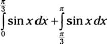
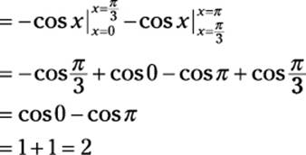
To evaluate this integral, break it into two integrals at the value of x where the asymptote is located:
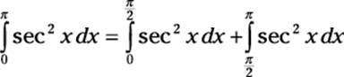
Now evaluate the sum of the two resulting integrals.
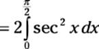
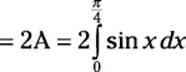
 You can save yourself a lot of work by noticing when two regions are symmetrical. In this case, the asymptote at
 ![]() splits the shaded area into two symmetrical regions. So you can find one integral and then double it to get your answer:
splits the shaded area into two symmetrical regions. So you can find one integral and then double it to get your answer:
Now use the steps from the previous section to evaluate this integral:
1. Express the integral as the limit of an integral:
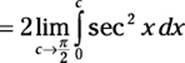
In this case, the vertical asymptote is at the upper limit of integration, so c approaches ![]() from the left — that is, from inside the interval where you’re measuring the area.
from the left — that is, from inside the interval where you’re measuring the area.
2. Evaluate the integral:
![]()
3. Evaluate the limit:
Note that tan![]() is undefined, because the function tan x has an asymptote at
is undefined, because the function tan x has an asymptote at ![]() , so the limit does not exist (DNE). Therefore, the integral that you’re trying to evaluate also does not exist because the area that it represents is infinite.
, so the limit does not exist (DNE). Therefore, the integral that you’re trying to evaluate also does not exist because the area that it represents is infinite.
Solving Area Problems with More Than One Function
The definite integral allows you to find the signed area under any interval of a single function. But when you want to find an area defined by more than one function, you need to be creative and piece together a solution. Professors love these problems as exam questions, because they test your reasoning skills as well as your calculus knowledge.
Fortunately, when you approach problems of this type correctly, you find that they’re not terribly difficult. The trick is to break down the problem into two or more regions that you can measure by using the definite integral, and then you use addition or subtraction to find the area that you’re looking for.
In this section, I get you up to speed on problems that involve more than one definite integral.
Finding the area under more than one function
Sometimes, a single geometric area is described by more than one function. For example, suppose that you want to find the shaded area shown in Figure 9-3.
Figure 9-3:Finding the area under y = sin xand y = cos xfrom 0 to ![]() .
.
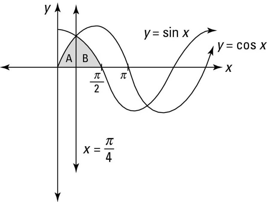
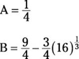
The first thing to notice is that the shaded area isn’t under a single function, so you can’t expect to use a single integral to find it. Instead, the region labeled A is under y = sin x and the region labeled B is under y = cos x. First, set up an integral to find the area of both of these regions:
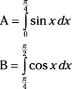
Now set up an equation to find their combined area:
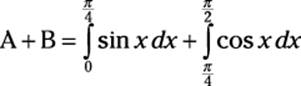
At this point, you can evaluate each of these integrals separately. But there’s an easier way.
 Because region A and region B are symmetrical, they have the same area. So you can find their combined area by doubling the area of a single region:
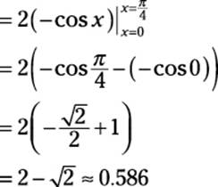
I choose to double region A because the integral limits of integration are easier, but doubling region B also works. Now integrate to find your answer:
Finding the area between two functions
To find an area between two functions, you need to set up an equation with a combination of definite integrals of both functions. For example, suppose that you want to calculate the shaded area in Figure 9-4.
Figure 9-4:Finding the area between y = x2and ![]() .
.
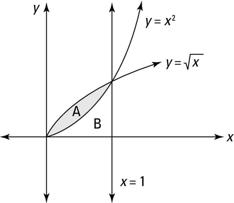
First, notice that the two functions y = x2 and ![]() intersect where x = 1. This information is important because it enables you to set up two definite integrals to help you find region A:
intersect where x = 1. This information is important because it enables you to set up two definite integrals to help you find region A:
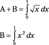
Although neither equation gives you the exact information that you’re looking for, together they help you out. Just subtract the second equation from the first as follows:
With the problem set up properly, now all you have to do is evaluate the two integrals:
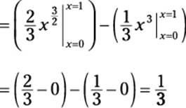
So the area between the two curves is ![]() .
.
As another example, suppose that you want to find the shaded area in Figure 9-5.
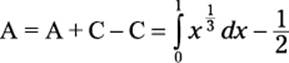
This time, the shaded area is two separate regions, labeled A and B. Region A is bounded above by ![]() and bounded below by y = x. However, for region B, the situation is reversed, and the region is bounded above by y = x and bounded below by
and bounded below by y = x. However, for region B, the situation is reversed, and the region is bounded above by y = x and bounded below by ![]() . I also label region C and region D, both of which figure into the problem.
. I also label region C and region D, both of which figure into the problem.
Figure 9-5:Finding the area between y = xand ![]() .
.
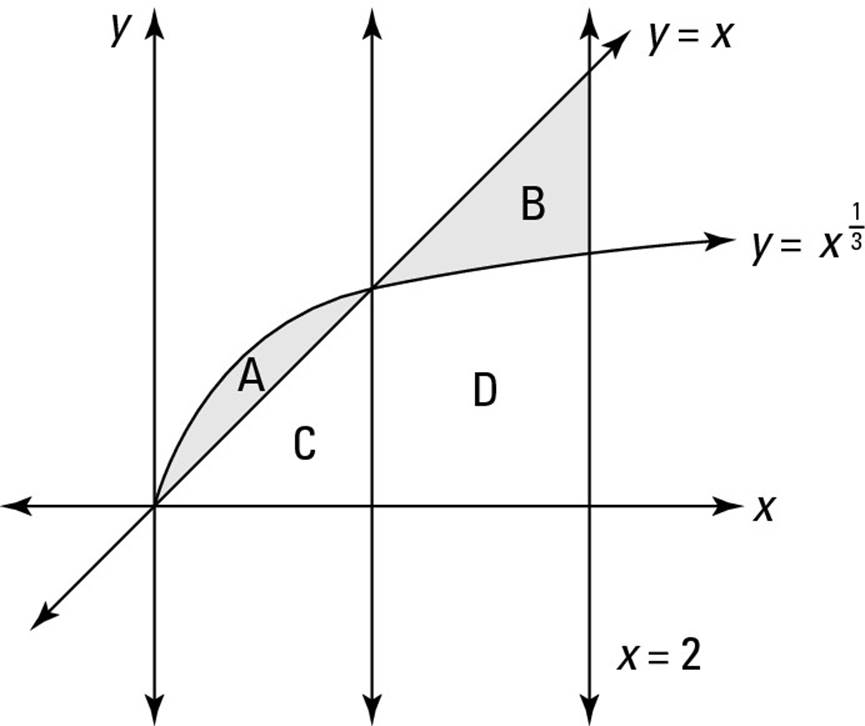
The first important step is finding where the two functions intersect — that is, where the following equation is true:
![]()
Fortunately, it’s easy to see that x = 1 satisfies this equation.
Now you want to build a few definite integrals to help you find the areas of region A and region B. Here are two that can help with region A:
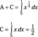
Notice that I evaluate the second definite integral without calculus, using simple geometry as I show you in Chapter 1. This is perfectly valid and a great time-saver.
Subtracting the second equation from the first provides an equation for the area of region A:
Now build two definite integrals to help you find the area of region B:
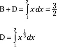
This time, I evaluate the first definite integral by using geometry instead of calculus. Subtracting the second equation from the first gives an equation for the area of region B:
![]()
Now you can set up an equation to solve the problem:
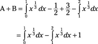
At this point, you’re forced to do some calculus:
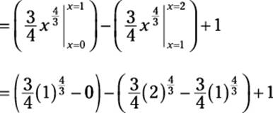
The rest is just arithmetic:
Looking for a sign
The solution to a definite integral gives you the signed area of a region (see Chapter 3 for more). In some cases, signed area is what you want, but in some problems you’re looking for unsigned area.
The signed area above the x-axis is positive, but the signed area below the x-axis is negative. In contrast, unsigned area is always positive. The concept of unsigned area is similar to the concept of absolute value. So if it’s helpful, think of unsigned area as the absolute value of a definite integral.
In problems where you’re asked to find the area of a shaded region on a graph, you’re looking for unsigned area. But if you’re unsure whether a question is asking you to find signed or unsigned area, ask the professor. This goes double if an exam question is unclear. Most professors will answer clarifying questions, so don’t be shy to ask.
Suppose that you’re asked to calculate the shaded unsigned area that’s shown in Figure 9-6.
This area is actually the sum of region A, which is above the x-axis, and region B, which is below it. To solve the problem, you need to find the sum of the unsigned areas of these two regions.
Figure 9-6:Finding the area between y = x2 –1 and y = 1 – x4.
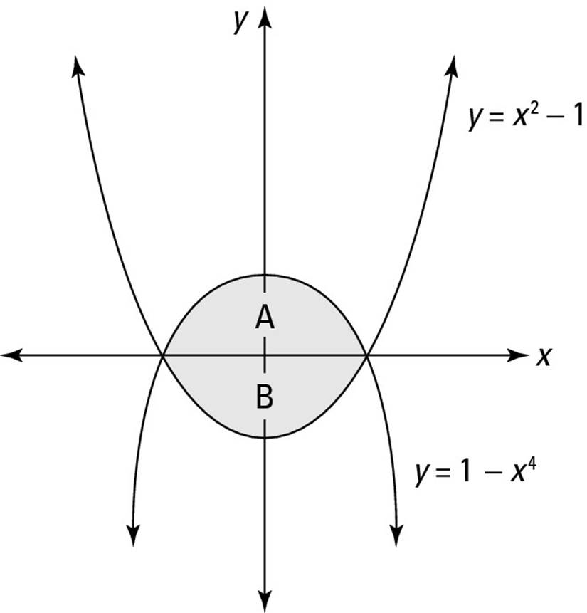
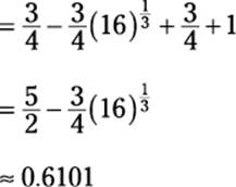
Fortunately, both functions intersect each other and the x-axis at the same two values of x: x = –1 and x = 1. Set up definite integrals to find the area of each region as follows:
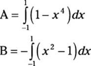
Notice that I negate the definite integral for region B to account for the fact that the definite integral produces negative area below the x-axis. Now just add the two equations together:
![]()
Solving this equation gives you the answer that you’re looking for (be careful with all those minus signs!):
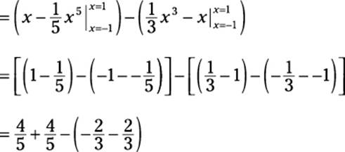
Notice at this point that the expression in the parentheses — representing the signed area of region B — is negative. But the minus sign outside the parentheses automatically flips the sign as intended:
![]()
Measuring unsigned area between curves with a quick trick
After you understand the concept of measuring unsigned area (which I discuss in the previous section), you’re ready for a trick that makes measuring the area between curves very straightforward. As I say earlier in this chapter, professors love to stick these types of problem on exams. So here’s a difficult exam question that’s worth spending some time with.
Find the unsigned shaded area in Figure 9-7. Approximate your answer to two decimal places using ![]() .
.
Figure 9-7:Finding the area between y = 4x – x2 and y = sin xfrom x = 0 to x = 4.
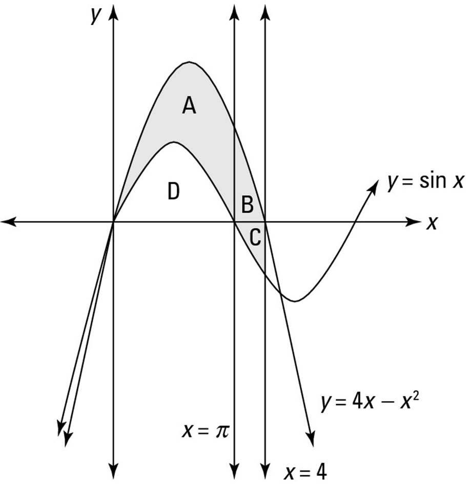
The first step is to find an equation for the solution (which will probably give you partial credit), and then worry about solving it.
I split the shaded area into three regions labeled A, B, and C. I also label region D, which you need to consider. Notice that x = π separates regions A and B, and the x-axis separates regions B and C.
You could find three separate equations for regions A, B, and C, but there’s a better way.
To measure the unsigned area between two functions, use this quick trick:
Area = Integral of top function – Integral of bottom function
That’s it! Instead of measuring the area above and below the x-axis, just plug the two integrals into this formula. In this problem, the top function is 4x – x2 and the bottom function is sin x:
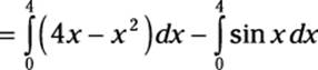
This evaluation isn’t too horrible:
When you get to this point, you can already see that you’re on track, because the professor was nice enough to give you an approximate value for cos 4:
![]()
So the unsigned area between the two functions is approximately 9.02 units.
 If the two functions change positions — that is, the top becomes the bottom and the bottom becomes the top — you may need to break the problem up into regions, as I show you earlier in this chapter. But even in this case, you can still save a lot of time by using this trick.
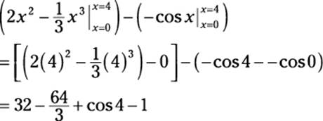
For example, earlier in this chapter, in “Finding the area between two functions,” I measure the shaded area from Figure 9-5 using four separate regions. Here’s how to do it using the trick in this section.
Notice that the two functions cross at x = 1. So from 0 to 1, the top function is ![]() and from 1 to 2 the top function is x. So set up two separate equations, one for region A and another for the region B:
and from 1 to 2 the top function is x. So set up two separate equations, one for region A and another for the region B:
When the calculations are complete, you get the following values for A and B:
Add these two values together to get your answer:
![]()
As you can see, the top-and-bottom trick gets you the same answer much more simply than measuring regions.
The Mean Value Theorem for Integrals
The Mean Value Theorem for Integrals guarantees that for every definite integral, a rectangle with the same area and width exists. Moreover, if you superimpose this rectangle on the definite integral, the top of the rectangle intersects the function. This rectangle, by the way, is called the mean-value rectangle for that definite integral. Its existence allows you to calculate the average value of the definite integral.
 Calculus boasts two Mean Value Theorems — one for derivatives and one for integrals. This section discusses the Mean Value Theorem for Integrals. You can find out about the Mean Value Theorem for Derivatives in Calculus For Dummies by Mark Ryan (Wiley).
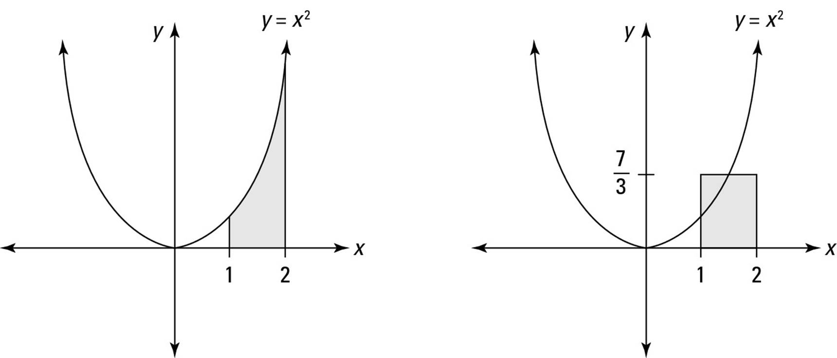
The best way to see how this theorem works is with a visual example. The first graph in Figure 9-8 shows the region described by the definite integral ![]() This region obviously has a width of 1, and you can evaluate it easily to show that its area is
This region obviously has a width of 1, and you can evaluate it easily to show that its area is ![]()
The second graph in Figure 9-8 shows a rectangle with a width of 1 and an area of ![]() It should come as no surprise that this rectangle’s height is also
It should come as no surprise that this rectangle’s height is also ![]() so the top of this rectangle intersects the original function.
so the top of this rectangle intersects the original function.
Figure 9-8: A definite integral and its mean-value rectangle have the same width and area.
The fact that the top of the mean-value rectangle intersects the function is mostly a matter of common sense. After all, the height of this rectangle represents the average value that the function attains over a given interval. This value must fall someplace between the function’s maximum and minimum values on that interval.
Here’s the formal statement of the Mean Value Theorem for Integrals: If f(x) is a continuous function on the closed interval [a, b], then there exists a number c in that interval such that:
![]()
This equation may look complicated, but it’s basically a restatement of this familiar equation for the area of a rectangle:
Area = Height · Width
In other words, start with a definite integral that expresses an area, and then draw a rectangle of equal area with the same width (b – a). The height of that rectangle — f(c) — is such that its top edge intersects the function where x = c.
The value f(c) is the average value of f(x) over the interval [a, b]. You can calculate it by rearranging the equation stated in the theorem:
![]()
For example, here’s how you calculate the average value of the shaded area in Figure 9-9:
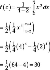
Figure 9-9: The definite integral ![]() and its mean-value rectangle.
and its mean-value rectangle.
Not surprisingly, the average value of this integral is 30, a value between the function’s minimum of 8 and its maximum of 64.
Calculating Arc Length
The arc length of a function on a given interval is the length from the starting point to the ending point as measured along the graph of that function.
In a sense, arc length is similar to the practical measurement of driving distance. For example, you may live only 5 miles from work “as the crow flies,” but when you check your odometer, you may find that the actual drive is closer to 7 miles. Similarly, the straight-line distance between two points is always less than the arc length along a curved function that connects them.
Using the formula, however, often involves trig substitution (see Chapter 7 for a refresher on this method of integration).
The formula for the arc length along a function y = f(x) from a to b is as follows:
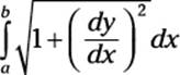
For example, suppose that you want to calculate the arc length along the function y = x2 from the point where x = 0 to the point where x = 2 (see Figure 9-10).
Figure 9-10:Measuring the arc length along y = x2 from (0, 0) to (2, 4).
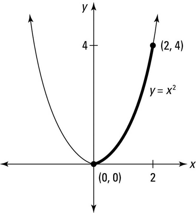
Before you begin, notice that if you draw a straight line between these two points, (0, 0) and (2, 4), its length is ![]() . So the arc length should be slightly greater.
. So the arc length should be slightly greater.
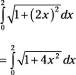
To calculate the arc length, first find the derivative of the function x2:
![]()
Now plug this derivative and the limits of integration into the formula as follows:
Calculating arc length usually gives you an opportunity to practice trig substitution — in particular, the tangent case. When you draw your trig substitution triangle, place ![]() on the hypotenuse, 2x on the opposite side, and 1 on the adjacent side. This gives you the following substitutions:
on the hypotenuse, 2x on the opposite side, and 1 on the adjacent side. This gives you the following substitutions:
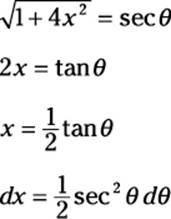
The result is this integral:
![]()
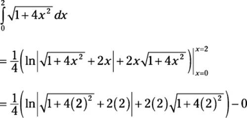
Notice that I remove the limits of integration because I plan to change the variable back to x before computing the definite integral. I spare you the details of calculating this indefinite integral, but you can see them in Chapter 7. Here’s the result:
![]()
Now write each sec θ and tan θ in terms of x:
![]()
At this point, I’m ready to evaluate the definite integral that I left off earlier:
You can either take my word that the second part of this substitution works out to 0 or you can calculate it yourself. To finish up: