Calculus II For Dummies, 2nd Edition (2012)

Part V. Advanced Topics

In this part . . .

You get a glimpse of what lies beyond Calculus II. I give you an overview of the next two semesters of math: Calculus III (the study of calculus in three or more dimensions) and Differential Equations (equations with derivatives mixed in as variables).

Chapter 14. Multivariable Calculus

In This Chapter

Visualizing vectors

Making the leap from two to three dimensions

Understanding cylindrical and spherical coordinates

Using partial derivatives

Space, as Captain Kirk says during the opening credits of the television series Star Trek, is the final frontier. Multivariable calculus (also known as Calculus III) focuses on techniques for doing calculus in space — that is, in three dimensions.

Mathematicians have a variety of terms for three dimensions: 3-D, 3-space, and R³ are the most common. Whatever you call it, adding a dimension makes multivariable calculus more interesting and useful, but also a bit trickier than single variable calculus.

In this chapter, I give you a quick introduction to multivariable calculus, touching on the highlights usually taught in a Calculus III class. First, I show you how vectors provide a method for linking a value with a direction. Next, I introduce you to three different 3-D coordinate systems: 3-D Cartesian coordinates, cylindrical coordinates, and spherical coordinates.

Building on this understanding of 3-D, I discuss functions of more than one variable, focusing on the function of two variables z = f(x, y). With an understanding of multivariable functions, I proceed to introduce you to the two most important concepts in multivariable calculus: partial derivatives and multiple integrals. By the end of this chapter, you’ll have a great platform from which to begin Calculus III.

Visualizing Vectors

Vectors are used to link a real number (called a scalar) with a direction on the plane or in space. They’re useful for navigation, where knowing what direction you’re sailing or flying in is important. Vectors also get a lot of play in physics, where forces that push and pull are also directional. And, as you may have guessed, Calculus III is chock full of vectors.

In this section, I introduce you to vectors. Although I keep this discussion in two dimensions, vectors are commonly used in three dimensions as well.

Understanding vector basics

A simple way to think of a vector is as an arrow that has both length and direction. By convention, a vector starts at the origin of the Cartesian plane (0, 0) and extends a certain length in some direction. Figure 14-1 shows a variety of vectors.

Figure 14-1:Vectors starting at the origin are distinguished by their endpoints.

As you can see, when a vector begins at the origin, its two components (its x and y values) correspond to the Cartesian coordinates of its endpoint. For example, the vector that begins at (0, 0) and ends at (3, 1) is distinguished as the vector <3, 1>.

Don’t confuse a vector <x, y> with its corresponding Cartesian pair (x, y), which is just a point.

By convention, vectors are labeled in books with boldfaced lowercase letters: a, b, c, and so forth (see Figure 14-1). But when you’re working with vectors on paper, most teachers are happy to see you replace the boldface with a little line or arrow over the letter.

Displacing a vector from the origin doesn’t change its value. For example, Figure 14-2 shows the vector <2, 3> with a variety of starting points.

Figure 14-2: All vectors with the same length and direction are equivalent, regardless of where they start.

Calculate the coordinates of a vector starting at (x₁, y₁) and ending at (x₂, y₂) as <x₂ – x₁, y₂ – y₁>. For example, here’s how to calculate the coordinates of vectors g, h, and i in Figure 14-2:

g = <0 – –2, 4 – 1> = <2, 3>

h = <–2 – –4, –1 – –4> = <2, 3>

i = <2 – 0, 1 – –2> = <2, 3>

As you can see, regardless of the starting and ending points, these vectors are all equivalent to each other and to f.

What’s in a name?

A scalar is just a fancy word for a real number. The name arises because a scalar scales a vector — that is, it changes the scale of a vector. For example, the real number 2 scales the vector v by a factor of 2 so that 2v is twice as long as v. You find out more about scalar multiplication in “Calculating with vectors.”

Distinguishing vectors and scalars

Just as Eskimos have tons of words for snow and Italians have even more words for pasta, mathematicians have bunches of words for real numbers. When you began algebra, you found out quickly that a constant or a coefficientwas just a real number in a specific context.

Similarly, when you’re discussing vectors and want to refer to a real number, use the word scalar. Only the name is different — deep in its heart, a scalar knows only too well that it’s just a good old-fashioned real number.

Some types of vector calculations produce new vectors, while others result in scalars. As I introduce these calculations throughout the next section, I tell you whether to expect a vector or a scalar as a result.

Calculating with vectors

Vectors are commonly used to model forces such as wind, sea current, gravity, and electromagnetism. Vector calculations are essential for all sorts of problems where forces collide. In this section, I give you a taste of how some simple calculations with vectors are accomplished.

Calculating magnitude

The length of a vector is called its magnitude. The notation for absolute value (| |) is also used for the magnitude of a vector. For example, |v| refers to magnitude of the vector v. (By the way, some textbooks represent magnitude with double bars [|| ||] instead of single bars. Either way, the meaning is the same.)

Calculate the magnitude of a vector v = <x, y> by using a variation of the distance formula. This formula is itself a variation of the trusty Pythagorean theorem:

For example, calculate the magnitude of the vector n = <4, –3> as follows:

As you can see, the use of the absolute value bars for the magnitude of vectors is appropriate: Magnitude, like all other distances, is always measured as a nonnegative value. The magnitude of a vector is the distance from the origin of a graph to its tip, just as the absolute value of a number is the distance from 0 on a number line to that number.

To measure the magnitude of a vector that doesn’t begin at the origin, use the magnitude formula. Here is the formula for the magnitude of a vector that begins at the point (x₁,y₁) and ends at the point (x₂, y₂) — you may note its similarity to the distance formula from Algebra I:

The magnitude of a vector is a scalar.

Scalar multiplication

Multiplying a vector by a scalar is called scalar multiplication. To perform scalar multiplication, multiply the scalar by each component of the vector. Here’s how you multiply the vector v = <x, y> by the scalar k:

kv = k<x, y> = <kx, ky>

For example, here’s how you multiply the vector p = <3, 5> by the scalars 2, –4, and :

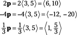
When you multiply a vector by a scalar, the result is a vector.

Geometrically speaking, scalar multiplication achieves the following:

Scalar multiplication by a positive number other than 1 changes the magnitude of the vector but not its direction.

Scalar multiplication by –1 reverses its direction but doesn’t change its magnitude.

Scalar multiplication by any other negative number both reverses the direction of the vector and changes its magnitude.

Scalar multiplication can change the magnitude of a vector by either increasing it or decreasing it.

Scalar multiplication by a number greater than 1 or less than –1 increases the magnitude of the vector.

Scalar multiplication by a fraction between –1 and 1 decreases the magnitude of the vector.

For example, the vector 2p is twice as long as p, the vector p is half as long as p, and the vector –p is the same length as p but extends in the opposite direction from the origin (as shown in Figure 14-3).

Figure 14-3:Scalar multiplication of a vector changes its magnitude and/or its direction.

Finding the unit vector

Every vector has a corresponding unit vector, which has the same direction as that vector but a magnitude of 1. To find the unit vector u of the vector v = <x, y>, divide that vector by its magnitude as follows:

Note that this formula uses scalar multiplication, as I show you in the preceding section, because the numerator is a vector and the denominator is a scalar.

As you may guess from its name, the unit vector is a vector.

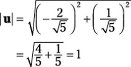
For example, to find the unit vector u of the vector q = <–2, 1>, first calculate its magnitude |q| as I show you earlier in this section:

Now use the previous formula to calculate the unit vector:

You can check that the magnitude of resulting vector u really is 1 as follows:

Adding and subtracting vectors

Add and subtract vectors component by component, as follows:

<x₁, y₁> + <x₂, y₂> = <x₁ + x₂, y₁ + y₂>

<x₁, y₁> – <x₂, y₂> = <x₁ – x₂, y₁ – y₂>

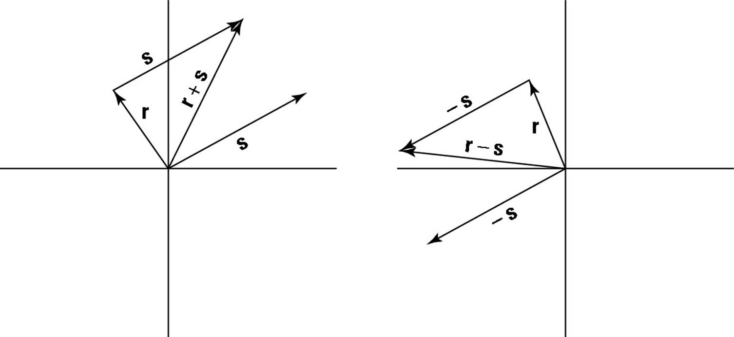
For example, if r = <–1, 3> and s = <4, 2>, here’s how to add and subtract these vectors:

r + s = <–1, 3> + <4, 2> = <–1 + 4, 3 + 2> = <3, 5>

r – s = <–1, 3> – <4, 2> = <–1 – 4, 3 – 2> = <–5, 1>

When you add or subtract two vectors, the result is a vector.

Geometrically speaking, the net effects of vector addition and subtraction are shown in Figure 14-4. In this example, the endpoint of r + s is equivalent to the endpoint of s when s begins at the endpoint of r. Similarly, the endpoint of r – s is equivalent to the endpoint of –s — that is, <–4, –2> — when –s begins at the endpoint of r.

Leaping to Another Dimension

Multivariable calculus is all about three (or more) dimensions. In this section, I show you three important systems for plotting points in 3-D.

Understanding 3-D Cartesian coordinates

The three-dimensional (3-D) Cartesian coordinate system (also called 3-D rectangular coordinates) is the natural extension of the 2-D Cartesian graph. The key difference is the addition of a third axis, the z-axis, extending perpendicularly through the origin.

Drawing a 3-D graph in two dimensions is kind of tricky. To get a better sense about how to think in 3-D, hold up Figure 14-5 where you can compare it with the interior corner of a room (not a round room!). Note the following:

The x-axis corresponds to where the left-hand wall meets the floor.

The y-axis corresponds to where the right-hand wall meets the floor.

The z-axis corresponds to where the two walls meet.

Just as the 2-D Cartesian graph is divided into four quadrants, the 3-D graph is divided into eight octants. From your perspective as you look at the graph, you’re standing inside the first octant, where all values of x, y, and z are positive.

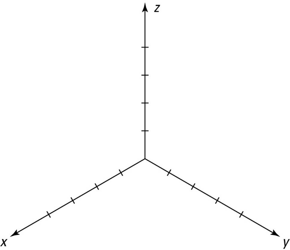
Figure 14-6 shows the complete 3-D Cartesian system with the point (1, 2, 5) plotted. In similarity with regular Cartesian coordinates, you plot this point by counting 1 unit in the positive x direction, and then 2 units in the positive y direction, and finally 5 units in the positive z direction.

Figure 14-6:Plotting the point (1, 2, 5) on the 3-D Cartesian coordinate system.

Using alternative 3-D coordinate systems

In Chapter 2, I discuss polar coordinates, an alternative to the Cartesian graph. Polar coordinates are useful because they allow you to express and solve a variety of problems more easily than Cartesian coordinates.

In this section, I show you two alternatives to the 3-D Cartesian coordinate system: cylindrical coordinates and spherical coordinates. As with polar coordinates, both of these systems give you greater flexibility to solve a wider range of problems.

Cylindrical coordinates

You probably remember polar coordinates from Pre-Calculus or maybe even Calculus I. Like the Cartesian coordinate system, the polar coordinate system assigns a pairing of values to every point on the plane. Unlike the Cartesian coordinate system, however, these values aren’t dependent on two perpendicular axes (though these axes are often drawn in to make the graph more readable). The key axis is the horizontal axis, which corresponds to the positive x-axis in Cartesian coordinates.

While a Cartesian pair is of the form (x, y), polar coordinates use (r, θ). Cylindrical coordinates are simply polar coordinates with the addition of a vertical z-axis extending from the origin, as in 3-D Cartesian coordinates (see “Understanding 3-D Cartesian coordinates” earlier in this chapter). Every point in space is assigned a set of cylindrical coordinates of the form (r, θ, z).

Here’s what you need to know:

The variable r measures the distance from the z-axis to that point.

The variable θ measures angular distance from the horizontal axis. This angle is measured in radians rather than degrees so that 2π = 360°. (See Chapter 2 for more about radians.)

The variable z measures the distance from that point to the xy-plane.

When plotting cylindrical coordinates, plot the first coordinates (r and θ) just as you would for polar coordinates (see Chapter 2). Then plot the z-coordinate as you would for 3-D Cartesian coordinates.

Figure 14-7 shows you how to plot the point (3, , 2) in cylindrical coordinates:

1. Count 3 units to the right of the origin on the horizontal axis (as you would when plotting polar coordinates).

2. Travel counterclockwise along the arc of a circle until you reach the line drawn at a -angle from the horizontal axis (again, as with polar coordinates).

3. Count 2 units above the plane and plot your point there.

Figure 14-7:Plotting the point (3, , 2) in cylindrical coordinates.

Spherical coordinates

Spherical coordinates are used — with slight variation — to measure latitude, longitude, and altitude on the most important sphere of them all, the planet Earth.

Every point in space is assigned a set of spherical coordinates of the form (ρ, θ, ϕ). In case you’re not in a sorority or fraternity, ρ is the lowercase Greek letter rho, θ is the lowercase Greek letter theta (commonly used in math to represent an angle), ϕ is the lower-case Greek letter phi, which is commonly pronounced either “fee” or “fye” (but never “foe” or “fum”).

The coordinate ρ corresponds to altitude. On the Earth, altitude is measured as the distance above or below sea level. In spherical coordinates, however, altitude indicates how far in space a point is from the origin.

The coordinate θ corresponds to longitude: a measurement of angular distance from the horizontal axis.

The coordinate ϕ corresponds to latitude. On the Earth, latitude is measured as angular distance from the equator. In spherical coordinates, however, latitude is measured as the angular distance from the north pole.

Plotting ϕ can be tricky at first. To get a feel for it, picture a globe and imagine traveling up and down along a single longitude line. Notice that as you travel, your latitude keeps changing, so

At the north pole, ϕ = 0

At the equator, ϕ =

At the south pole, ϕ = π

Some textbooks substitute the Greek letter ρ (rho) for r. Either way, the coordinate means the same thing: altitude, which is the distance of a point from the origin. In other textbooks, the order of the last two coordinates is changed around. Make sure you know which convention your book uses.

Figure 14-8 shows you how to plot a point in spherical coordinates. For

example, suppose you want to plot the point (4, , ). Follow these steps to do that:

1. Count 4 units outward in the positive direction from the origin on the horizontal axis.

2. Travel counterclockwise along the arc of a circle until you reach the line drawn at a -angle from the horizontal axis (again, as with polar coordinates).

3. Imagine a single longitude line arcing from the north pole of a sphere through the point on the equator where you are right now and onward to the south pole.

4. Travel down to the line of latitude at an angular distance of from the north pole — that is, halfway between the equator and the south pole — and plot your point there.

Figure 14-8:Plotting the point (4, , ) in spherical coordinates.

Functions of Several Variables

You know from algebra that a function y = f(x) is basically a mathematical machine for turning one number into another. The variable x is the input variable and y is the output variable so that every value of x gives you no more than one y value.

When you graph a curve, you can use the vertical-line test to make sure it’s a function: Any vertical line that intersects a function intersects it at exactly one point, as illustrated in Figure 14-9.

These concepts related to functions also carry over into functions of more than one variable. For example, here are some functions of two variables:

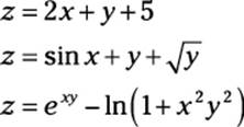
The general form for a function of two variables is z = f(x, y). Every function of two variables takes a Cartesian pair (x, y) as its input and in turn outputs a z value. Looking at the three previous examples, plugging in the input (0, 1) gives you an output of 6 for the first function, 2 for the second function, and 1 for the third.

Figure 14-9:The vertical-line test shows that a function outputs no more than one y value for every inputted xvalue.

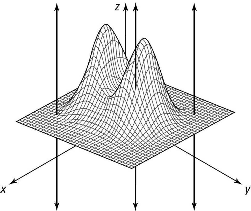
A good way to visualize a function of two variables is as a surface floating over the xy-plane in a 3-D Cartesian graph. (True, this surface can cross the plane and continue below it — just as a function can cross the x-axis — but for now, just picture it floating.) Every point on this surface looms directly above exactly one point on the plane. That is, if you pass a vertical line through any point on the plane, it crosses the function at no more than one point. Figure 14-10 illustrates this concept.

The concept of a function can be extended to higher dimensions. For example, w = f(x, y, z) is the basic form for a function of three variables. Because this function (as well as other functions of more than two variables) exists in more than three dimensions, it’s a lot harder to picture. For now, just concentrate on making the leap from two to three dimensions — that is, from functions of one variable to functions of two variables. Most of the multivariable calculus that you study in Calculus III is in three dimensions. (Maybe it should be called Calculus 3-D.)

Partial Derivatives

Partial derivatives are the higher-dimensional equivalent of the derivatives that you know from Calculus I. Just as a derivative represents the slope of a function on the Cartesian plane, a partial derivative represents a similar concept of slope in higher dimensions. In this section, I clarify this notion of slope in three dimensions. I also show you how to calculate the partial derivatives of functions of two variables.

Measuring slope in three dimensions

In the earlier section “Functions of Several Variables,” I recommend that you visualize a function of two variables z = f(x, y) as a surface floating over the xy-plane of a 3-D Cartesian graph. (See Figure 14-10 for a picture of a sample function.)

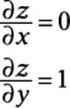
For example, take the function z = y, as shown in Figure 14-11. As you can see, this function looks a lot like the sloped roof of a house. Imagine yourself standing on this surface. When you walk parallel with the y-axis, your altitude either rises or falls. In other words, as the value of y changes so does the value of z. But when you walk parallel with the x-axis, your altitude remains the same; changing the value of x has no effect on z.

So intuitively, you expect that the partial derivative — the slope in the direction of the y-axis — is 1. You also expect that the partial derivative — the slope in the direction of the x-axis — is 0. In the next section, I show you how to calculate partial derivatives to verify this result.

Figure 14-11:The function z = y.

Evaluating partial derivatives

Evaluating partial derivatives isn’t much more difficult than evaluating regular derivatives. Given a function z(x, y), the two partial derivatives are and . Here’s how you calculate them:

To calculate , treat y as a constant and use x as your differentiation variable.

To calculate , treat x as a constant and use y as your differentiation variable.

For example, suppose you’re given the equation z = 5x²y³. To find , treat y as if it were a constant — that is, treat the entire factor 5y³ as if it’s one big coefficient — and differentiate x²:

To find , treat x as if it were a constant — that is, treat 5x² as if it’s the coefficient — and differentiate y³:

As another example, suppose that you’re given the equation z = 2e^x sin y + ln x.

To find , treat y as if it were a constant and differentiate by the variable x:

To find , treat x as if it were a constant and differentiate by the variable y:

As you can see, when differentiating by y, the ln x term is treated as a constant and drops away completely.

Returning to the example from the previous section — the “sloped-roof” function z = y — here are both partial derivatives of this function:

As you can see, this calculation produces the predicted results.

Multiple Integrals

You already know that an integral allows you to measure area in two dimensions (see Chapter 1 if this concept is unclear). And as you probably know from solid geometry, the analog of area in three dimensions is volume.

Multiple integrals are the higher-dimensional equivalent of the good old-fashioned integrals that you discover in Calculus II. They allow you to measure volume in three dimensions (or more).

Most of the multiple integrals that you’ll ever have to solve come in two varieties: double integrals and triple integrals. In this section, I show you how to understand and calculate both of these types of multiple integrals.

Measuring volume under a surface

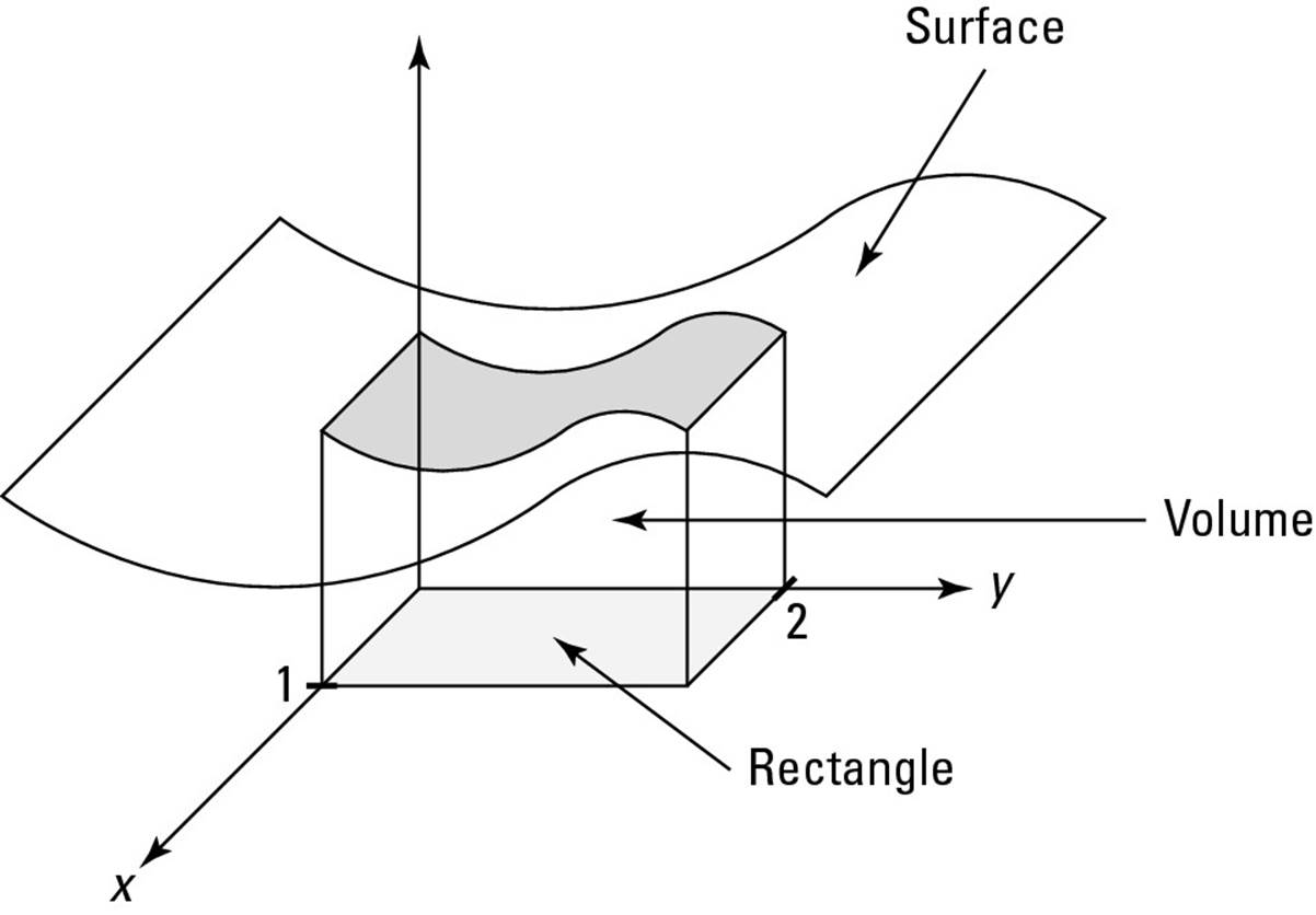
Definite integrals provide a reliable way to measure the signed area between a function and the x-axis as bounded by any two values of x. (I cover this in detail in Chapters 1 and 3.) Similarly, a double integral allows you to measure the signed volume between a function z = f(x, y) and the xy-plane as bounded by any two values of x and any two values of y.

Here’s an example of a double integral:

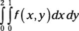
Although it may look complicated, a double integral is really an integral inside another integral. To help you see this, I bracket off the inner integral in the previous example:

When you focus on the integral inside the brackets, you can see that the limits of integration for 0 and 1 correspond with the dx — that is, x = 0 and x = 1. Similarly, the limits of integration 0 and 2 correspond with the dy — that is, y = 0 and y = 2.

To get a picture of this volume, look at Figure 14-12. The double integral measures the volume between f(x, y) and the xy-plane as bounded by a rectangle. In this case, the rectangle is described by the four lines x = 0, x = 1, y = 0, and y = 2.

Evaluating multiple integrals

Multiple integrals (double integrals, triple integrals, and so forth) are usually definite integrals, so evaluating them results in a real number. Evaluating multiple integrals is similar to evaluating nested functions: You work them from the inside out.

Solving double integrals

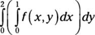
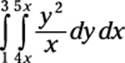
Solve double integrals in two steps: First evaluate the inner integral, and then plug this solution into the outer integral and solve that. For example, suppose you want to integrate the following double integral:

To start out, place the inner integral in parentheses so you can better see what you’re working with:

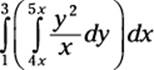
Now focus on what’s inside the parentheses. For the moment, you can ignore the rest. Your integration variable is y, so treat the variable x as if it were a constant, moving it outside the integral:

Notice that the limits of integration in this integral are functions of x. So the result of this definite integral will also be a function of x:

Now plug this expression into the outer integral. In other words, substitute it for what’s inside the parentheses:

Evaluate this integral as usual:

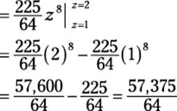
Making sense of triple integrals

Triple integrals look scary, but if you take them step by step, they’re no more difficult than regular integrals. As with double integrals, start in the center and work your way out. For example:

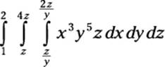
Begin by separating the two inner integrals:

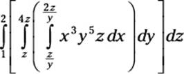
Your plan of attack is to evaluate the integral in the brackets first, and then the integral in the braces, and finally the outer integral. First things first:

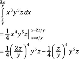
Notice that plugging in values for x results in an expression in terms of y and z. Now simplify this expression to make it easier to work with:

Plug this solution back in to replace the bracketed integral:

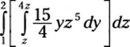
One integral down, two to go. This time, focus on the integral inside the braces. This time, the integration variable is y:

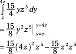
Again, simplify before proceeding:

Plug this result back into the integral as follows:

Now evaluate this integral: