Calculus II For Dummies, 2nd Edition (2012)
Part I. Introduction to Integration

In this part . . .
I give you an overview of Calculus II, plus a review of Pre-Calculus and Calculus I. You discover how to measure the areas of weird shapes by using a new tool: the definite integral. I show you the connection between differentiation, which you know from Calculus I, and integration. And you see how this connection provides a useful way to solve area problems.
Chapter 1. An Aerial View of the Area Problem
In This Chapter
![]() Measuring the area of shapes by using classical and analytic geometry
Measuring the area of shapes by using classical and analytic geometry
![]() Understanding integration as a solution to the area problem
Understanding integration as a solution to the area problem
![]() Building a formula for calculating definite integrals using Riemann sums
Building a formula for calculating definite integrals using Riemann sums
![]() Applying integration to the real world
Applying integration to the real world
![]() Considering sequences and series
Considering sequences and series
![]() Looking ahead at some advanced math
Looking ahead at some advanced math
Humans have been measuring the area of shapes for thousands of years. One practical use for this skill is measuring the area of a parcel of land. Measuring the area of a square or a rectangle is simple, so land tends to get divided into these shapes.
Discovering the area of a triangle, circle, or polygon is also easy, but as shapes get more unusual, measuring them gets harder. Although the Greeks were familiar with the conic sections — parabolas, ellipses, and hyperbolas — they couldn’t reliably measure shapes with edges based on these figures.
Descartes’s invention of analytic geometry — studying lines and curves as equations plotted on a graph — brought great insight into the relationships among the conic sections. But even analytic geometry didn’t answer the question of how to measure the area inside a shape that includes a curve.
In this chapter, I show you how integral calculus (integration for short) developed from attempts to answer this basic question, called the area problem. With this introduction to the definite integral, you’re ready to look at the practicalities of measuring area. The key to approximating an area that you don’t know how to measure is to slice it into shapes that you do know how to measure (for example, rectangles).
Slicing things up is the basis for the Riemann sum, which allows you to turn a sequence of closer and closer approximations of a given area into a limit that gives you the exact area that you’re seeking. I walk you through a step-by-step process that shows you exactly how the formal definition for the definite integral arises intuitively as you start slicing unruly shapes into nice, crisp rectangles.
Checking Out the Area
Finding the area of certain basic shapes — squares, rectangles, triangles, and circles — is easy. But a reliable method for finding the area of shapes containing more esoteric curves eluded mathematicians for centuries. In this section, I give you the basics of how this problem, called the area problem, is formulated in terms of a new concept, the definite integral.
The definite integral represents the area of a region bounded by the graph of a function, the x-axis, and two vertical lines located at the limits of integration. Without getting too deep into the computational methods of integration, I give you the basics of how to state the area problem formally in terms of the definite integral.
Comparing classical and analytic geometry
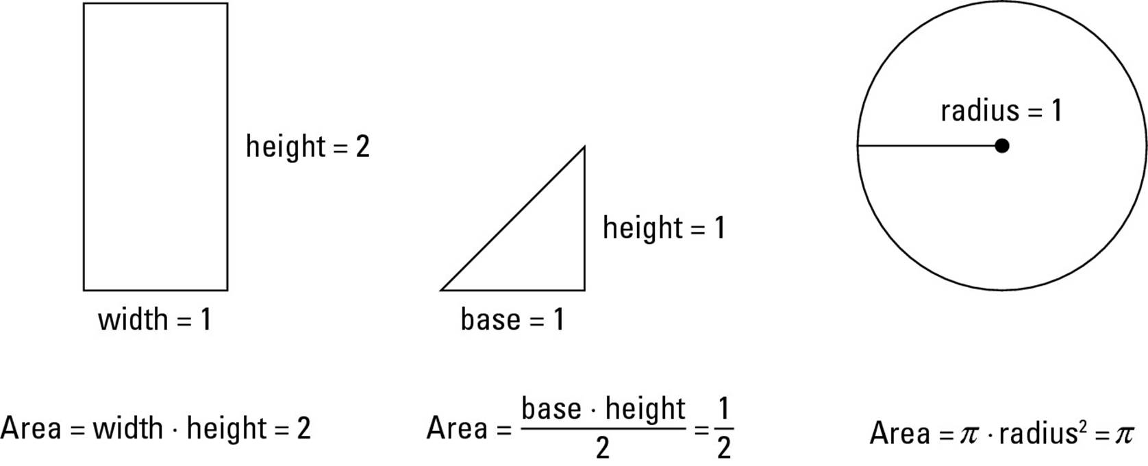
In classical geometry, you discover a variety of simple formulas for finding the area of different shapes. For example, Figure 1-1 shows the formulas for the area of a rectangle, a triangle, and a circle.
Figure 1-1:Formulas for the area of a rectangle, a triangle, and a circle.
Wisdom of the ancients
Long before calculus was invented, the ancient Greek mathematician Archimedes used his method of exhaustion to calculate the exact area of a segment of a parabola. Indian mathematicians also developed quadrature methods for some difficult shapes before Europeans began their investigations in the 17th century.
These methods anticipated some of the methods of calculus. But before calculus, no single theory could measure the area under arbitrary curves.
When you move on to analytic geometry — geometry on the Cartesian graph — you gain new perspectives on classical geometry. Analytic geometry provides a connection between algebra and classical geometry. You find that circles, squares, and triangles — and many other figures — can be represented by equations or sets of equations, as shown in Figure 1-2.
Figure 1-2: A rectangle, a triangle, and a circle embedded on the graph.
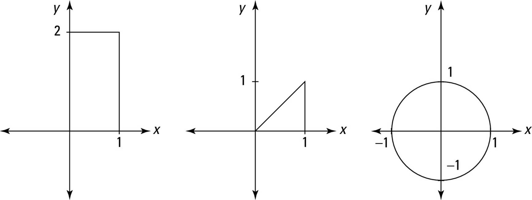
You can still use the trusty old methods of classical geometry to find the areas of these figures. But analytic geometry opens up more possibilities — and more problems.
Discovering a new area of study
Figure 1-3 illustrates three curves that are much easier to study with analytic geometry than with classical geometry: a parabola, an ellipse, and a hyperbola.
Figure 1-3: A parabola, an ellipse, and a hyperbola embedded on the graph.
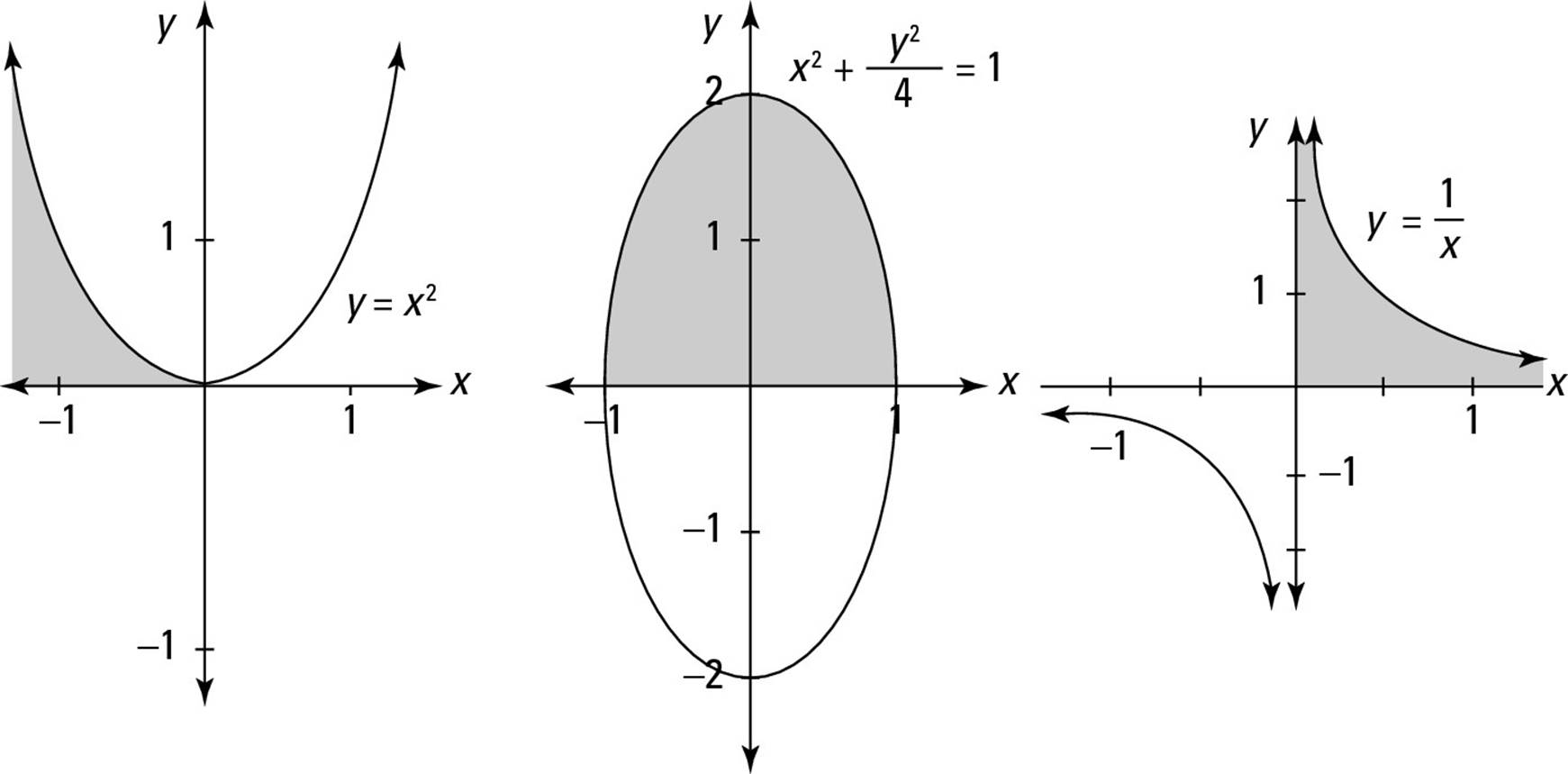
Analytic geometry gives a very detailed account of the connection between algebraic equations and curves on a graph. But analytic geometry doesn’t tell you how to find the shaded areas shown in Figure 1-3.
Figure 1-4 shows three more equations placed on the graph: a sine curve, an exponential curve, and a logarithmic curve.
Figure 1-4: A sine curve, an exponential curve, and a logarithmic curve embedded on the graph.
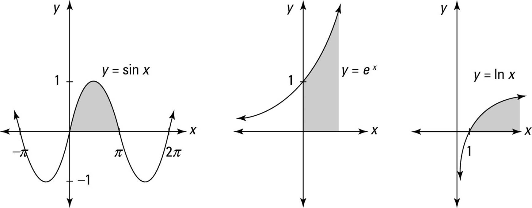
Again, analytic geometry provides a connection between these equations and how they appear as curves on the graph. But it doesn’t tell you how to find any of the shaded areas in Figure 1-4.
Generalizing the area problem
Notice that in all the examples in the previous section, I shade each area in a very specific way. Above, the area is bounded by a function. Below, it’s bounded by the x-axis. And on the left and right sides, the area is bounded by vertical lines (though in some cases, you may not notice these lines because the function crosses the x-axis at this point).
You can generalize this problem to study any continuous function. To illustrate this, the shaded region in Figure 1-5 shows the area under the function f(x) between the vertical lines x = a and x = b.
Figure 1-5: A typical area problem.
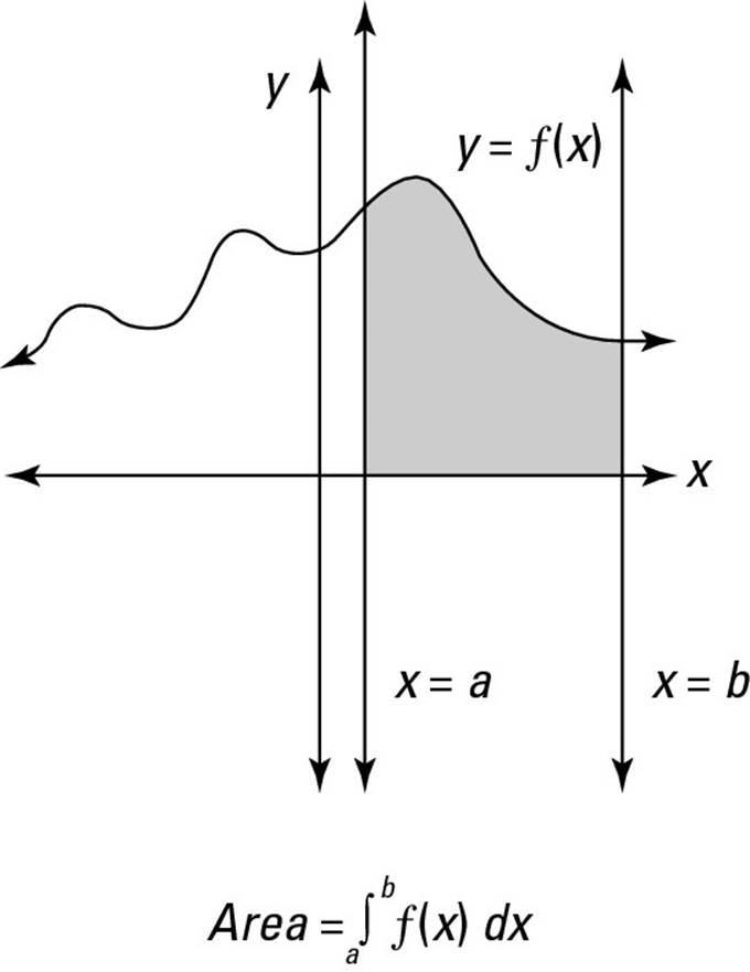
The area problem is all about finding the area under a continuous function between two constant values of x that are called the limits of integration, usually denoted by a and b.
 The limits of integration aren’t limits in the sense that you learned about in Calculus I. They’re simply constants that tell you the width of the area that you’re attempting to measure.
In a sense, this formula for the shaded area isn’t much different from those that I provide earlier in this chapter. It’s just a formula, which means that if you plug in the right numbers and calculate, you get the right answer.
The catch, however, is in the word calculate. How exactly do you calculate using this new symbol ![]() ? As you may have figured out, the answer is on the cover of this book: calculus. To be more specific, integral calculus, or integration.
? As you may have figured out, the answer is on the cover of this book: calculus. To be more specific, integral calculus, or integration.
Most typical Calculus II courses taught at your friendly neighborhood college or university focus on integration — the study of how to solve the area problem. When Calculus II gets confusing (and to be honest, you probably will get confused somewhere along the way), try to relate what you’re doing to this central question: “How does what I’m working on help me find the area under a function?”
Finding definite answers with the definite integral
You may be surprised to find out that you’ve known how to integrate some functions for years without even knowing it. (Yes, you can know something without knowing that you know it.)
For example, find the rectangular area under the function y = 2 between x = 1 and x = 4, as shown in Figure 1-6.
Figure 1-6: The rectangular area under the function y = 2, between x = 1 and x = 4.
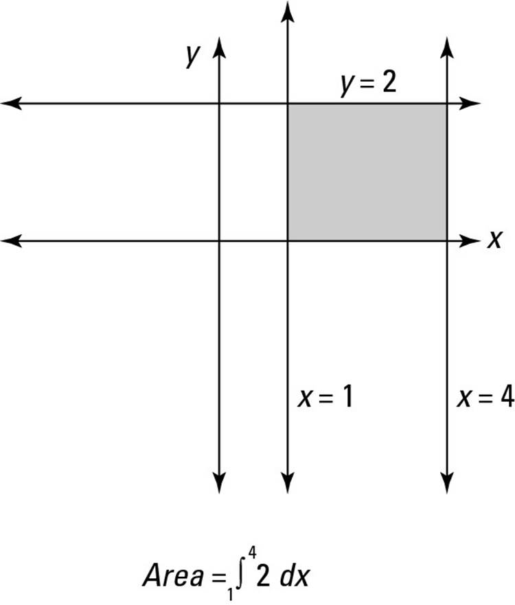
This is just a rectangle with a base of 3 and a height of 2, so its area is 6. But this is also an area problem that can be stated in terms of integration as follows:
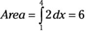
As you can see, the function I’m integrating here is f(x) = 2. The limits of integration are 1 and 4 (notice that the greater value goes on top). You already know that the area is 6, so you can solve this calculus problem without resorting to any scary or hairy methods. But, you’re still integrating, so please pat yourself on the back, because I can’t quite reach it from here.
The following expression is called a definite integral:
![]()
For now, don’t spend too much time worrying about the deeper meaning behind the ![]() symbol or the dx (which you may remember from your fond memories of the differentiating that you did in Calculus I). Just think of
symbol or the dx (which you may remember from your fond memories of the differentiating that you did in Calculus I). Just think of ![]() and dxas notation placed around a function — notation that means area.
and dxas notation placed around a function — notation that means area.
What’s so definite about a definite integral? Two things, really:
![]() You definitely know the limits of integration (in this case, 1 and 4). Their presence distinguishes a definite integral from an indefinite integral, which you find out about in Chapter 3. Definite integrals always include the limits of integration; indefinite integrals never include them.
You definitely know the limits of integration (in this case, 1 and 4). Their presence distinguishes a definite integral from an indefinite integral, which you find out about in Chapter 3. Definite integrals always include the limits of integration; indefinite integrals never include them.
![]() A definite integral definitely equals a number (assuming that its limits of integration are also numbers). This number may be simple to find or difficult enough to require a room full of math professors scribbling away with #2 pencils. But, at the end of the day, a number is just a number. And, because a definite integral is a measurement of area, you should expect the answer to be a number.
A definite integral definitely equals a number (assuming that its limits of integration are also numbers). This number may be simple to find or difficult enough to require a room full of math professors scribbling away with #2 pencils. But, at the end of the day, a number is just a number. And, because a definite integral is a measurement of area, you should expect the answer to be a number.
 When the limits of integration aren’t numbers, a definite integral doesn’t necessarily equal a number. For example, a definite integral whose limits of integration are k and 2k would most likely equal an algebraic expression that includes k. Similarly, a definite integral whose limits of integration are sin θ and 2 sin θ would most likely equal a trig expression that includes θ. To sum up, because a definite integral represents an area, it always equals a number — though you may or may not be able to compute this number.
As another example, find the triangular area under the function y = x, between x = 0 and x = 8, as shown in Figure 1-7.
This time, the shape of the shaded area is a triangle with a base of 8 and a height of 8, so its area is 32 (because the area of a triangle is half the base times the height). But again, this is an area problem that can be stated in terms of integration as follows:
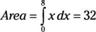
Figure 1-7: The triangular area under the function y = x, between x = 0 and x = 8.
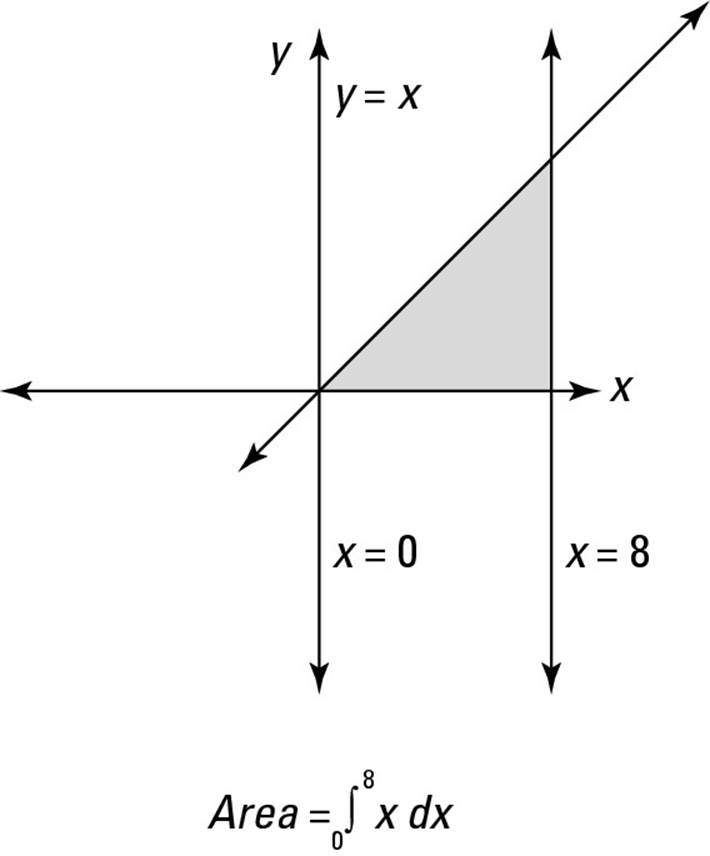
The function I’m integrating here is f(x) = x and the limits of integration are 0 and 8. Again, you can evaluate this integral with methods from classical and analytic geometry. And, again, the definite integral evaluates to a number, which is the area below the function and above the x-axis between x = 0 and x = 8.
As a final example, find the semicircular area between x = –4 and x = 4, as shown in Figure 1-8.
Figure 1-8: The semicircular area between x = –4 and x = 4.

First of all, remember from Pre-Calculus how to express the area of a circle with a radius of 4 units:
x2 + y2 = 16
Next, solve this equation for y:
![]()
A little basic geometry tells you that the area of the whole circle is 16π, so you know that the area of the shaded semicircle is 8π. Even though a circle isn’t a function (and remember that integration deals exclusively with continuous functions!), the shaded area in this case is beneath the top portion of the circle. The equation for this curve is the following function:
![]()
So you can represent this shaded area as a definite integral:
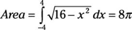
Again, the definite integral evaluates to a number, which is the area under the function between the limits of integration.
Slicing Things Up
One good way of approaching a difficult task — from planning a wedding to climbing Mount Everest — is to break it down into smaller and more manageable pieces.
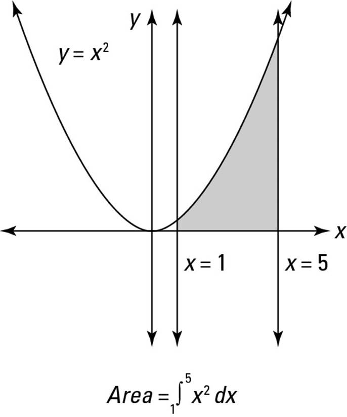
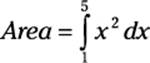
In this section, I show you the basics of how mathematician Bernhard Riemann used this same type of approach to calculate the definite integral, which I introduce in the earlier section “Checking Out the Area.” Throughout this section I use the example of the area under the function y = x2, between x = 1 and x = 5. You can find this example in Figure 1-9.
Figure 1-9: The area under the function y = x2, between x = 1 and x = 5.
Untangling a hairy problem using rectangles
The earlier section “Checking Out the Area” tells you how to write the definite integral that represents the area of the shaded region in Figure 1-9:
Unfortunately, this definite integral — unlike those earlier in this chapter — doesn’t respond to the methods of classical and analytic geometry that I use to solve the earlier problems. (If it did, integrating would be much easier and this book would be a lot thinner!)
Even though you can’t solve this definite integral directly (yet!), you can approximate it by slicing the shaded region into two pieces, as shown in Figure 1-10.
Figure 1-10:Area approximated by two rectangles.
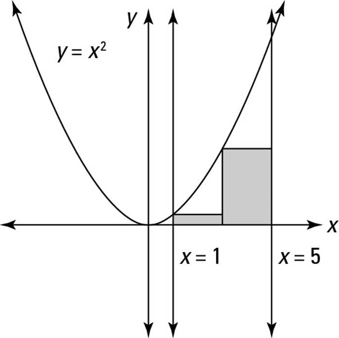
Obviously, the region that’s now shaded — it looks roughly like two steps going up but leading nowhere — is less than the area that you’re trying to find. Fortunately, these steps do lead someplace, because calculating the area under them is fairly easy.
Each rectangle has a width of 2. The tops of the two rectangles cut across where the function x2 meets x = 1 and x = 3, so their heights are 1 and 9, respectively. So the total area of the two rectangles is 20, because
2 (1) + 2 (9) = 2 (1 + 9) = 2 (10) = 20
With this approximation of the area of the original shaded region, here’s the conclusion you can draw:
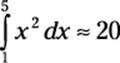
Granted, this is a ballpark approximation with a really big ballpark. But, even a lousy approximation is better than none at all. To get a better approximation, try cutting the figure that you’re measuring into a few more slices, as shown in Figure 1-11.
Figure 1-11: A closer approximation; the area is approximated by four rectangles.
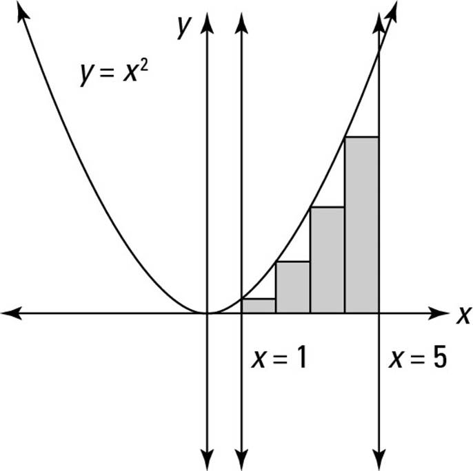
Again, this approximation is going to be less than the actual area that you’re seeking. This time, each rectangle has a width of 1. And the tops of the four rectangles cut across where the function x2 meets x = 1, x = 2, x = 3, and x= 4, so their heights are 1, 4, 9, and 16, respectively. So the total area of the four rectangles is 30, because
1 (1) + 1 (4) + 1 (9) + 1 (16) = 1 (1 + 4 + 9 + 16) = 1 (30) = 30
Therefore, here’s a second approximation of the shaded area that you’re seeking:
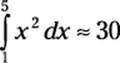
Your intuition probably tells you that your second approximation is better than your first, because slicing the rectangles more thinly allows them to cut in closer to the function. You can verify this intuition by realizing that both 20 and 30 are less than the actual area, so whatever this area turns out to be, 30 must be closer to it.
You might imagine that by slicing the area into more rectangles (say 10, or 100, or 1,000,000), you’d get progressively better estimates. And, again, your intuition would be correct: As the number of slices increases, the result approaches 41.3333 . . . .
In fact, you may very well decide to write:
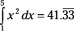
This, in fact, is the correct answer. But to justify this conclusion, you need a bit more rigor.
Building a formula for finding area
In the previous section, you calculate the areas of two rectangles and four rectangles, respectively, as follows:
How high is up?
When you’re slicing a weird shape into rectangles, finding the width of each rectangle is easy because they’re all the same width. You just divide the total width of the area that you’re measuring into equal slices.
Finding the height of each individual rectangle, however, requires a bit more work. Start by drawing the horizontal tops of all the rectangles you’ll be using. Then, for each rectangle follow these steps:
1. Locate where the top of the rectangle meets the function.
2. Find the value of x at that point by looking down at the x-axis directly below this point.
3. Get the height of the rectangle by plugging that x-value into the function.
2 (1) + 2 (9) = 2 (1 + 9) = 20
1 (1) + 1 (4) + 1 (9) + 1 (16) = 1 (1 + 4 + 9 + 16) = 30
Each time, you divide the area that you’re trying to measure into rectangles that all have the same width. Then you multiply this width by the sum of the heights of all the rectangles. The result is the area of the shaded area.
In general, then, the formula for calculating an area sliced into n rectangles is:
Area of rectangles = wh1 + wh2 + ... + whn
In this formula, w is the width of each rectangle and h1, h2, . . . , hn, and so forth are the various heights of the rectangles. When the width of all the rectangles is the same, you can simplify this formula as follows:
Area of rectangles = w (h1 + h2 + ... + hn)
Remember that as n increases — that is, the more rectangles you draw — the total area of all the rectangles approaches the area of the shape that you’re trying to measure.
I hope you agree that there’s nothing terribly tricky about this formula. It’s just basic geometry, measuring the area of rectangles by multiplying their widths and heights. Yet, in the rest of this section, I transform this simple formula into the following formula, called a Riemann sum formula for the definite integral:
![]()
No doubt about it, this formula is eye-glazing. That’s why I build it step by step by starting with the simple area formula. This way, you understand completely how all this fancy notation is really just an extension of what you can see for yourself.
If you’re sketchy on any of these symbols — such as Σ and the limit — read on, because I explain them as I go along. (For a more thorough review of these symbols, see Chapter 2.)
Approximating the definite integral
Earlier in this chapter I tell you that the definite integral means area. So in transforming the simple formula
Area of rectangles = w (h1 + h2 + ... + hn)
the first step is simply to introduce the definite integral:
![]()
As you can see, the = has been changed to ≈ — that is, the equation has been demoted to an approximation. This change is appropriate — the definite integral is the precise area inside the specified bounds, which the area of the rectangles merely approximates.
Limiting the margin of error
As n increases — that is, the more rectangles you draw — your approximation gets better and better. In other words, as n approaches infinity, the area of the rectangles that you’re measuring approaches the area that you’re trying to find.
So you may not be surprised to find that when you express this approximation in terms of a limit, you remove the margin of error and restore the approximation to the status of an equation:
![]()
This limit simply states mathematically what I say in the previous section: As n approaches infinity, the area of all the rectangles approaches the exact area that the definite integral represents.
Widening your understanding of width
The next step is to replace the variable w, which stands for the width of each rectangle, with an expression that’s more useful.
Remember that the limits of integration tell you the width of the area that you’re trying to measure, with a as the smaller value and b as the greater. So you can write the width of the entire area as b – a. And when you divide this area into n rectangles, each rectangle has the following width:
![]()
Substituting this expression into the approximation results in the following:
![]()
As you can see, all I’m doing here is expressing the variable w in terms of a, b, and n.
Summing things up with sigma notation
You may remember that sigma notation — the Greek symbol Σ used in equations — allows you to streamline equations that have long strings of numbers added together. Chapter 2 gives you a review of sigma notation, so check it out if you need a review.
The expression h1 + h2 + ... + hn is a great candidate for sigma notation:
![]()
So in the equation that you’re working with, you can make a simple substitution as follows:
![]()
Now I tweak this equation by placing ![]() inside the sigma expression (this is a valid rearrangement, as I explain in Chapter 2):
inside the sigma expression (this is a valid rearrangement, as I explain in Chapter 2):
![]()
Heightening the functionality of height
Remember that the variable hi represents the height of a single rectangle that you’re measuring. (The sigma notation takes care of adding up these heights.) The last step is to replace hi with something more functional. And functional is the operative word, because the function determines the height of each rectangle.
Here’s the short explanation, which I clarify later: The height of each individual rectangle is determined by a value of the function at some value of x lying someplace on that rectangle, so:
hi = f(xi*)
The notation xi*, which I explain further in “Moving left, right, or center,” means something like “an appropriate value of xi.” That is, for each hi in your sum (h1, h2, and so forth) you can replace the variable hi in the equation for an appropriate value of the function. Here’s how this looks:
![]()
This is the complete Riemann sum formula for the definite integral, so in a sense I’m done. But I still owe you a complete explanation for this last substitution, and here it comes.
Moving left, right, or center
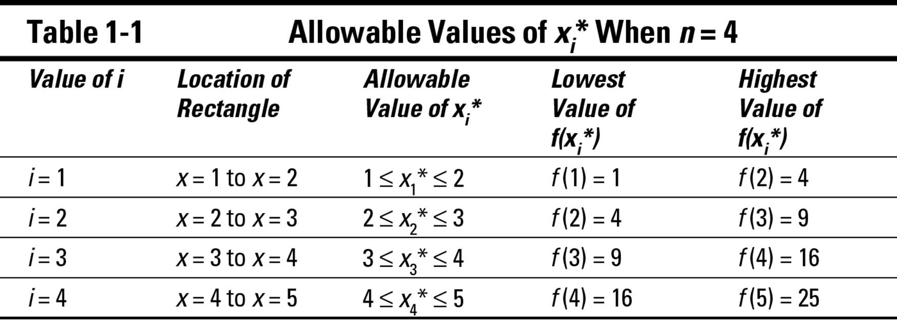
Go back to the example that I start with in the earlier section “Untangling a hairy problem using rectangles,” and take another look at the way I slice the shaded area into four rectangles in Figure 1-12.
Figure 1-12:Approximating area with left rectangles.
As you can see, the heights of the four rectangles are determined by the value of f(x) when x is equal to 1, 2, 3, and 4, respectively — that is, f(1), f(2), f(3), and f(4). Notice that the upper-left corner of each rectangle touches the function and determines the height of each rectangle.
However, suppose that I draw the rectangles as shown in Figure 1-13.
Figure 1-13:Approximating area with right rectangles.
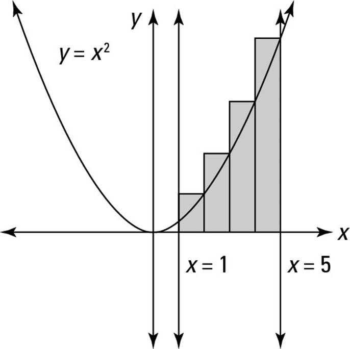
In this case, the upper-right corner touches the function, so the heights of the four rectangles are f(2), f(3), f(4), and f(5).
Now suppose that I draw the rectangles as shown in Figure 1-14.
Figure 1-14:Approximating area with midpoint rectangles.
This time, the midpoint of the top edge of each rectangle touches the function, so the heights of the rectangles are f(1.5), f(2.5), f(3.5), and f(4.5).
It seems that I can draw rectangles at least three different ways to approximate the area that I’m attempting to measure. They all lead to different approximations, so which one leads to the correct answer? The answer is all of them.
This surprising answer results from the fact that the equation for the definite integral includes a limit. No matter how you draw the rectangles, as long as the top of each rectangle coincides with the function at one point (at least), the limit smoothes over any discrepancies as n approaches infinity. This slack in the equation shows up as the * in the expression f(xi*).
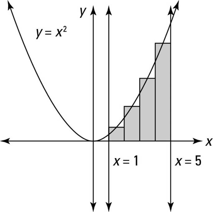
For instance, in the example that uses four rectangles, the first rectangle is located from x = 1 to x = 2, so
1 ≤ x1* ≤ 2 therefore 1 ≤ f(x1*) ≤ 4
Table 1-1 shows you the range of allowable values for xi when approximating this area with four rectangles. In each case, you can draw the height of the rectangle on a range of different values of x.
In Chapter 3, I discuss this idea — plus a lot more about the fine points of the formula for the definite integral — in greater detail.
Defining the Indefinite
The Riemann sum formula for the definite integral, which I discuss in the previous section, allows you to calculate areas that you can’t calculate by using classical or analytic geometry. The downside of this formula is that it’s quite a hairy beast. In Chapter 3, I show you how to use it to calculate area, but most students throw their hands up at this point and say, “There has to be a better way!”
The better way is called the indefinite integral. The indefinite integral looks a lot like the definite integral. Compare for yourself:
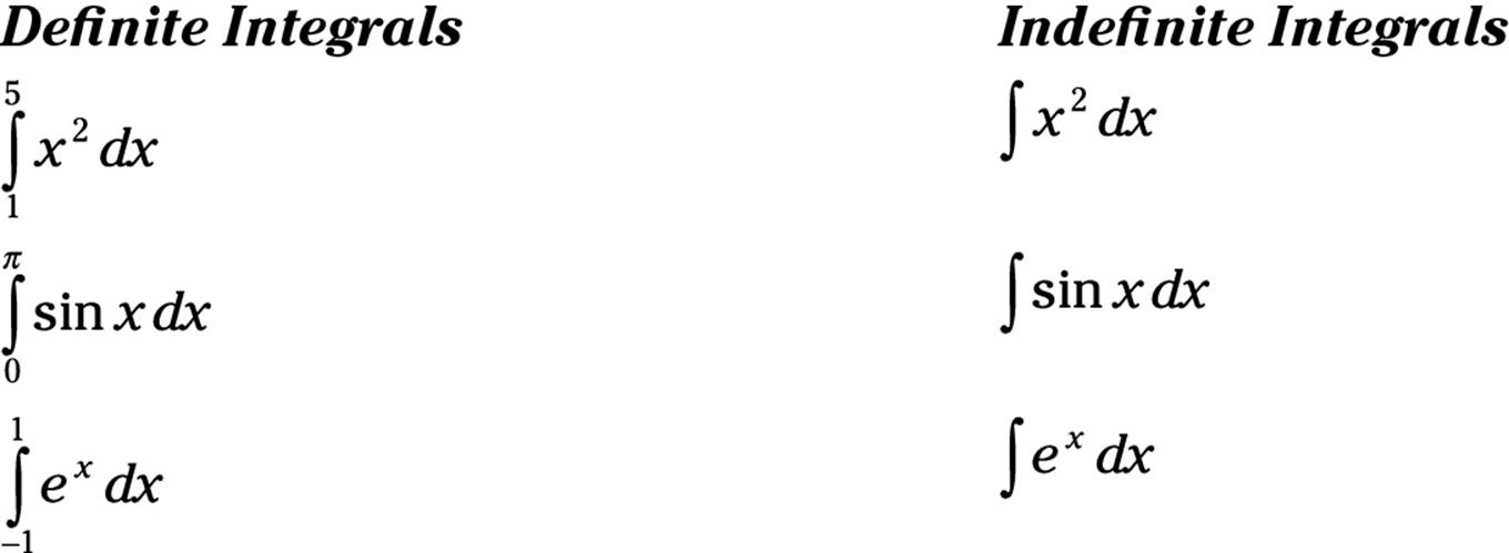
Like the definite integral, the indefinite integral is a tool for measuring the area under a function. Unlike it, however, the indefinite integral has no limits of integration, so evaluating it doesn’t give you a number. Instead, when you evaluate an indefinite integral, the result is a function that you can use to obtain all related definite integrals. Chapter 3 gives you the details of how definite and indefinite integrals are related.
Indefinite integrals provide a convenient way to calculate definite integrals. In fact, the indefinite integral is the inverse of the derivative, which you know from Calculus I. (Don’t worry if you don’t remember all about the derivative — Chapter 2 gives you a thorough review.) By inverse, I mean that the indefinite integral of a function is really the anti-derivative of that function. This connection between integration and differentiation is more than just an odd little fact: It leads to the Fundamental Theorem of Calculus (FTC).
For example, you know that the derivative of x2 is 2x. So you expect that the anti-derivative — that is, the indefinite integral — of 2x is x2. This is fundamentally correct with one small tweak, as I explain in Chapter 3.
Seeing integration as anti-differentiation allows you to solve tons of integrals without resorting to the Riemann sum formula (I tell you about this in Chapter 3). But integration can still be sticky depending on the function that you’re trying to integrate. Mathematicians have developed a wide variety of techniques for evaluating integrals. Some of these methods are variable substitution (see Chapter 5), integration by parts (see Chapter 6), trig substitution (see Chapter 7), and integration by partial fractions (see Chapter 8).
Solving Problems with Integration
After you understand how to describe an area problem using the definite integral (Part I), and how to calculate integrals (Part II), you’re ready to get into action solving a wide range of problems.
Some of these problems know their place and stay in two dimensions. Others rise up and create a revolution in three dimensions. In this section, I give you a taste of these types of problems, with an invitation to check out Part III of this book for a deeper look.
Three types of problems that you’re almost sure to find on an exam involve finding the area between curves, the length of a curve, and volume of revolution. I focus on these types of problems and many others in Chapters 9 and 10.
We can work it out: Finding the area between curves
When you know how the definite integral represents the area under a curve, finding the area between curves isn’t too difficult. Just figure out how to break the problem into several smaller versions of the basic area problem. For example, suppose that you want to find the area between the function y = sin x and y = cos x, from x = 0 to ![]() — that is, the shaded area A in Figure 1-15.
— that is, the shaded area A in Figure 1-15.
Figure 1-15:The area between the function y = sin x and y = cos x,from x = 0 to ![]() .
.
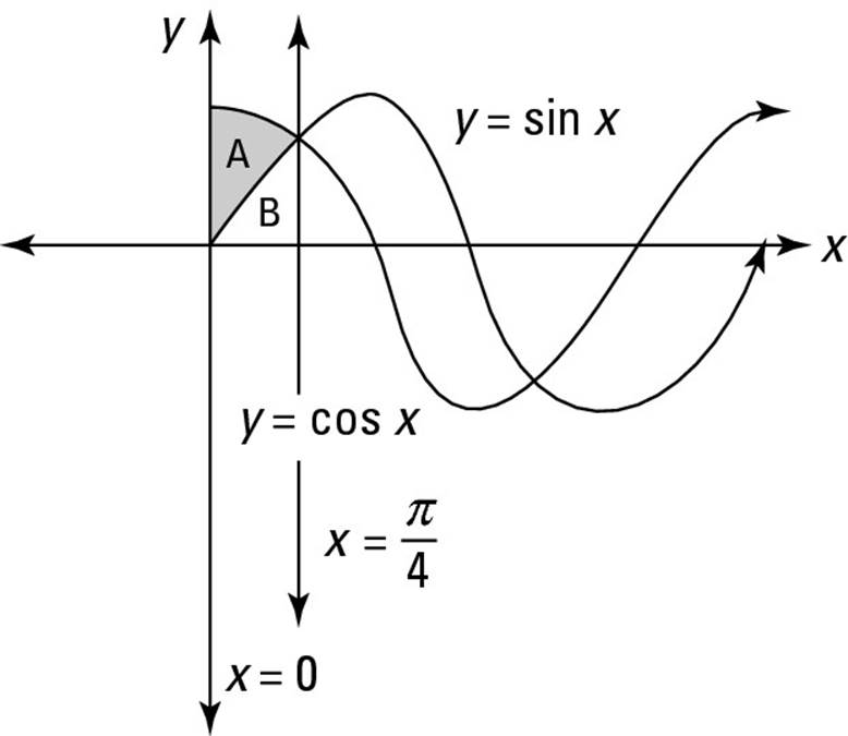
In this case, integrating y = cos x allows you to find the total area A + B. And integrating y = sin x gives you the area of B. So you can subtract A + B – B to find the area of A.
For more on how to find an area between curves, flip to Chapter 9.
Walking the long and winding road
Measuring a segment of a straight line or a section of a circle is simple when you’re using classical and analytic geometry. But how do you measure a length along an unusual curve produced by a polynomial, exponential, or trig equation?
For example, what’s the distance from Point A to Point B along the curve shown in Figure 1-16?
Figure 1-16:The distance from Point A to Point B along the function y = ln x.
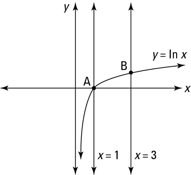
Once again, integration is your friend. In Chapter 9, I show you how integration provides a formula that allows you to measure arc length.
You say you want a revolution
Calculus also allows you to find the volume of unusual shapes. In most cases, calculating volume involves a dimensional leap into multivariable calculus, the topic of Calculus III, which I touch on in Chapter 14. But in a few situations, setting up an integral just right allows you to calculate volume by integrating over a single variable — that is, by using the methods you discover in Calculus II.
Among the trickiest of these problems involves the solid of revolution of a curve. In such problems, you’re presented with a region under a curve. You imagine the solid that results when you spin this region around the axis, and then you calculate the volume of this solid as seen in Figure 1-17.
Figure 1-17: A solid of revolution produced by spinning the function y = x2around the axis x = 0.
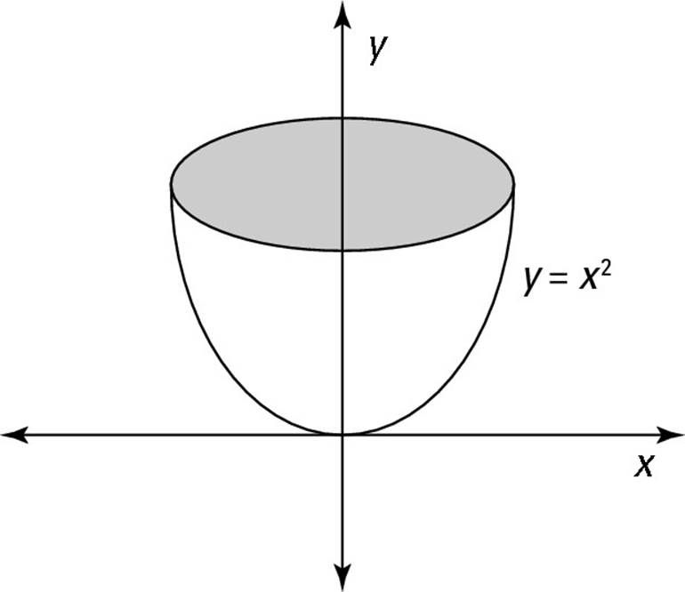
Clearly, you need calculus to find the area of this region. Then you need more calculus and a clear plan of attack to find the volume. I give you all this and more in Chapter 10.
Understanding Infinite Series
The last third of a typical Calculus II course — roughly five weeks — usually focuses on the topic of infinite series. I cover this topic in detail in Part IV. Here’s an overview of some of the ideas you find out about there.
Distinguishing sequences and series
A sequence is a string of numbers in a determined order. For example:
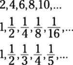
Sequences can be finite or infinite, but calculus deals well with the infinite, so it should come as no surprise that calculus concerns itself only with infinite sequences.
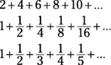
You can turn an infinite sequence into an infinite series by changing the commas into plus signs:
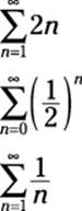
Sigma notation, which I discuss further in Chapter 2, is useful for expressing infinite series more succinctly:
Evaluating series
Evaluating an infinite series is often possible. That is, you can find out what all those numbers add up to. A helpful way to get a handle on some series is to create a related sequence of partial sums — that is, a sequence that includes the first term, the sum of the first two terms, the sum of the first three terms, and so forth. For example, here’s a sequence of partial sums for the second series shown earlier:
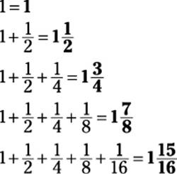
The resulting sequence of partial sums provides strong evidence of this conclusion:
![]()
Identifying convergent and divergent series
When a series evaluates to a number — as does ![]() — it’s called a convergent series. When a series isn’t convergent, it’s called a divergent series.
— it’s called a convergent series. When a series isn’t convergent, it’s called a divergent series.
Identifying whether a series is convergent or divergent isn’t always simple. For example, take another look at the third series I introduce earlier in this section:
![]()
This is called the harmonic series, but can you guess by looking at it whether it converges or diverges? (Before you begin adding fractions, let me warn you that the partial sum of the first 10,000 numbers is less than 10.)
An ongoing problem as you study infinite series is deciding whether a given series is convergent or divergent. Chapter 13 gives you a slew of tests to help you find out.
Advancing Forward into Advanced Math
Although it’s further along in math than many people dream of going, calculus isn’t the end but a beginning. Whether you’re enrolled in a Calculus II class or reading on your own, here’s a brief overview of some areas of math that lie beyond integration.
Multivariable calculus
Multivariable calculus generalizes differentiation and integration to three dimensions and beyond. Differentiation in more than two dimensions requires partial derivatives. Integration in more than two dimensions utilizes multiple integrals.
In practice, multivariable calculus as taught in most Calculus III classes is restricted to three dimensions, using three sets of axes and the three variables x, y, and z. I discuss multivariable calculus in more detail in Chapter 14.
Partial derivatives
As you know from Calculus I, a derivative is the slope of a curve at a given point on the graph. When you extend the idea of slope to three dimensions, a new set of issues that need to be resolved arises.
For example, suppose that you’re standing on the side of a hill that slopes upward. If you draw a line up and down the hill through the point you’re standing on, the slope of this line will be steep. But if you draw a line across the hill through the same point, the line will have little or no slope at all. (For this reason, mountain roads tend to cut sideways, winding their way up slowly, rather than going straight up and down.)
So when you measure slope on a curved surface in three dimensions, you need to take into account not only the point where you’re measuring the slope but the direction in which you’re measuring it. Partial derivatives allow you to incorporate this additional information.
Multiple integrals
Earlier in this chapter, you discover that integration allows you to measure the area under a curve. In three dimensions, the analog becomes finding the volume under a curved surface. Multiple integrals (integrals nested inside other integrals) allow you to compute such volume.
Differential equations
After multivariable calculus, the next topic most students learn on their precipitous math journey is differential equations.
Differential equations arise in many branches of science, including physics, where key concepts such as velocity and acceleration of an object are computed as first and second derivatives. The resulting equations contain hairy combinations of derivatives that are confusing and tricky to solve. For example:
![]()
Beyond ordinary differential equations, which include only ordinary derivatives, partial differential equations — such as the heat equation or the Laplace equation — include partial derivatives. For example:
![]()
I provide a look at ordinary and partial differential equations in Chapter 15.
Fourier analysis
So much of physics expresses itself in differential equations that finding reliable methods of solving these equations became a pressing need for 19th-century scientists. Mathematician Joseph Fourier met with the greatest success.
Fourier developed a method called Fourier analysis for expressing every function as the function of an infinite series of sines and cosines. Because these trig functions are continuous and infinitely differentiable, Fourier analysis provided a unified approach to solving huge families of differential equations that were previously incalculable.
Numerical analysis
A lot of math is theoretical and ideal: the search for exact answers without regard to practical considerations such as “How long will this problem take to solve?” (If you’ve ever run out of time on a math exam, you probably know what I’m talking about!)
In contrast, numerical analysis is the search for a close-enough answer in a reasonable amount of time. For example, here’s an integral that can’t be evaluated:
![]()
But even though you can’t solve this integral, you can approximate its solution to any degree of accuracy that you desire. And for real-world applications, a good approximation is often acceptable as long as you (or, more likely, a computer) can calculate it in a reasonable amount of time. Such a procedure for approximating the solution to a problem is called an algorithm.
Numerical analysis examines algorithms for qualities such as precision (the margin of error for an approximation) and tractability (how long the calculation takes for a particular level of precision).