Calculus II For Dummies, 2nd Edition (2012)

Part I. Introduction to Integration

Chapter 2. Dispelling Ghosts from the Past: A Review of Pre-Calculus and Calculus I

In This Chapter

Making sense of exponents of 0, negative numbers, and fractions

Graphing common continuous functions and their transformations

Remembering trig identities and sigma notation

Understanding and evaluating limits

Differentiating by using all your favorite rules

Remember Charles Dickens’s A Christmas Carol? You know, Scrooge and those ghosts from the past. Math can be just like that story: all the stuff you thought was dead and buried for years suddenly pays a spooky visit when you least expect it.

This quick review is designed to save you from any unnecessary sleepless nights. Before you proceed any further on your calculus quest, make sure that you’re on good terms with the information in this chapter.

First I cover all the Pre-Calculus you forgot to remember: polynomials, exponents, graphing functions and their transformations, trig identities, and sigma notation. Then I give you a brief review of Calculus I, focusing on limits and derivatives. I close the chapter with a topic that you may or may not know from Calculus I: L’Hopital’s Rule for evaluating indeterminate forms of limits.

If you still feel stumped after you finish this chapter, I recommend that you pick up a copy of Pre-Calculus For Dummies by Deborah Rumsey, PhD, or Calculus For Dummies by Mark Ryan (both published by Wiley), for a more in-depth review.

Forgotten but Not Gone: A Review of Pre-Calculus

Here’s a true story: When I returned to college to study math, my first degree having been in English, it had been a lot of years since I’d taken a math course. I won’t mention how many years, but when I confided this number to my first Calculus teacher, she swooned and was revived with smelling salts (okay, I’m exaggerating a little), and then she asked with a concerned look on her face, “Are you sure you’re up for this?”

I wasn’t sure at all, but I hung in there. Along the way, I kept refining a stack of notes labeled “Brute Memorization” — basically, what you find in this section. Here’s what I learned that semester: Whether it’s been one year or 20 since you took Pre-Calculus, make sure that you’re comfy with this information.

Knowing the facts on factorials

The factorial of a positive integer, represented by the symbol !, is that number multiplied by every positive integer less than itself. For example:

5! = 5 · 4 · 3 · 2 · 1 = 120

Notice that the factorial of every positive number equals that number multiplied by the next-lowest factorial. For example:

6! = 6 (5!)

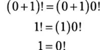
Generally speaking, then, the following equality is true:

(x + 1)! = (x + 1) x!

This equality provides the rationale for the odd-looking convention that 0! = 1:

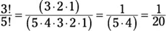
When factorials show up in fractions (as they do in Chapters 12 and 13), you can usually do a lot of cancellation that makes them simpler to work with. For example:

Even when a fraction includes factorials with variables, you can usually simplify it. For example:

Polishing off polynomials

A polynomial is any function of the following form:

f(x) = a_nxⁿ + a_n–1x^n–1 + a_n–2x^n–2 + ... + a₁x + a₀

Note that every term in a polynomial is x raised to the power of a nonnegative integer, multiplied by a real-number coefficient. Here are a few examples of polynomials:

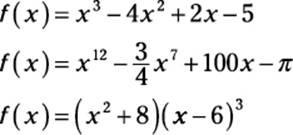
Note that in the last example, multiplying the right side of the equation will change the polynomial to a more recognizable form.

Polynomials enjoy a special status in math because they’re particularly easy to work with. For example, you can find the value of f(x) for any x value by plugging this value into the polynomial. Furthermore, polynomials are also easy to differentiate and integrate. Knowing how to recognize polynomials when you see them will make your life in any math course a whole lot easier.

Powering through powers (exponents)

Remember when you found out that any number (except 0) raised to the power of 0 equals 1? That is:

n⁰ = 1 (for all n ≠ 0)

It just seemed weird, didn’t it? But when you asked your teacher why, I suspect you got an answer that sounded something like “That’s just how mathematicians define it.” Not a very satisfying answer, is it?

However if you’re absolutely dying to know why (or if you’re even mildly curious about it), the answer lies in number patterns.

For starters, suppose that n = 2. Table 2-1 is a simple chart that encapsulates information you already know.

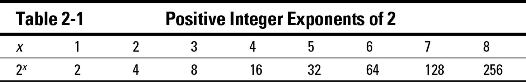
As you can see, as x increases by 1, 2x doubles. So, as x decreases by 1, 2x is halved. You don’t need rocket science to figure out what happens when x = 0. Table 2-2 shows you what happens.

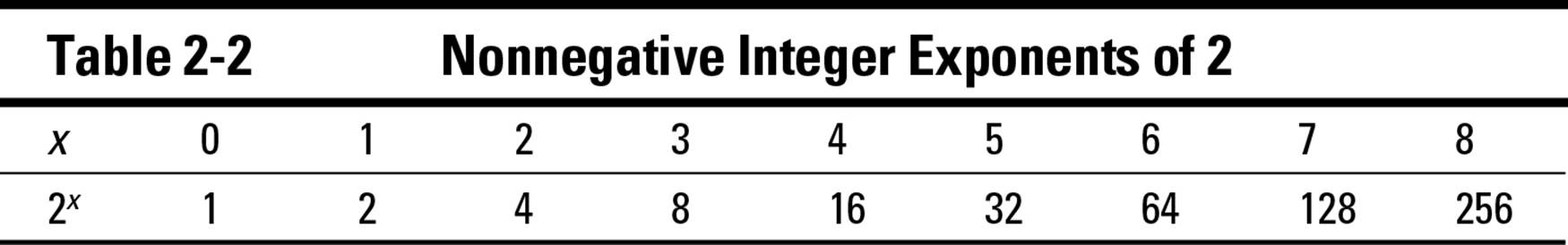
This chart provides a simple rationale of why 2⁰ = 1. The same reasoning works for all other real values of n (except 0). Furthermore, Table 2-3 shows you what happens when you continue the pattern into negative values of x.

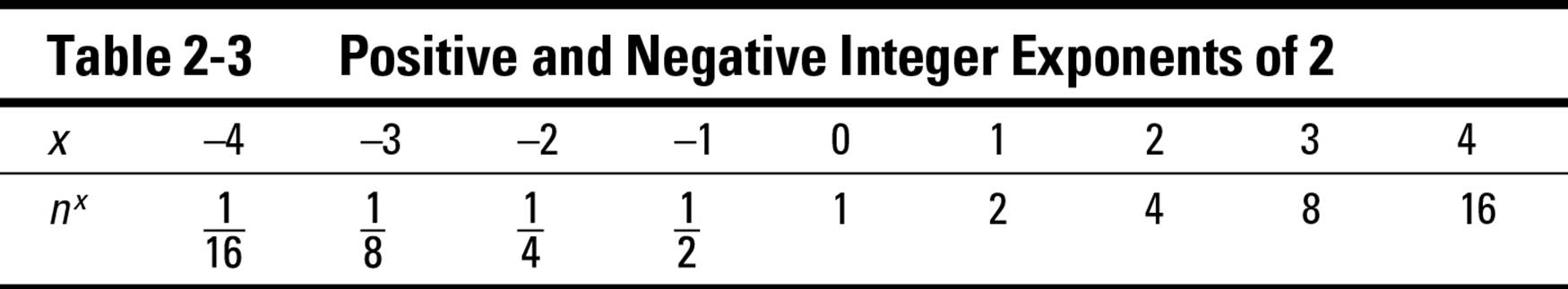
As the table shows, . This pattern also holds for all real, nonzero values of n, so

Notice from this table that the following rule holds:

n^an^b = n^{a + b}

For example:

2³ · 2⁴ = 2^{3 + 4} = 2⁷ = 128

This rule allows you to evaluate fractional exponents as roots. For example:

You can generalize this rule for all bases and fractional exponents as follows:

Plotting these values for x and f(x) = 2^x onto a graph provides an even deeper understanding. Check out Figure 2-1.

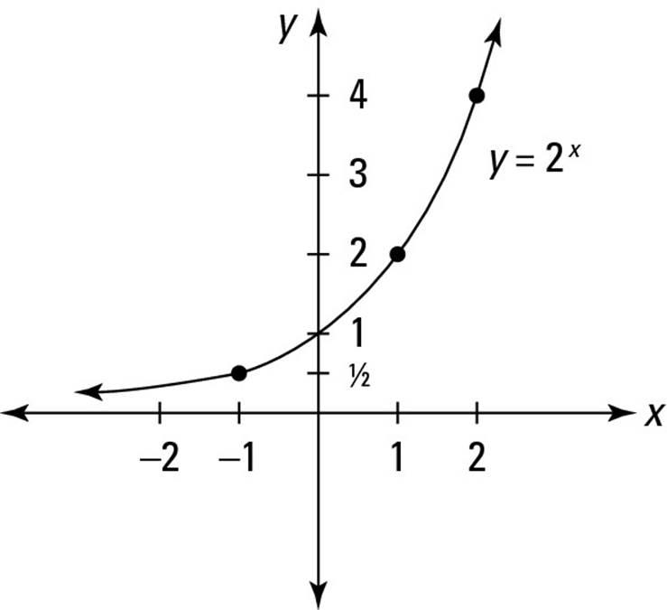
In fact, assuming the continuity of the exponential curve even provides a rationale (or, I suppose, an irrationale) for calculating a number raised to an irrational exponent. This calculation is beyond the scope of this book, but it’s a problem in numerical analysis, a topic that I discuss briefly in Chapter 1.

Noting trig notation

Trigonometry is a big and important subject in Calculus II. I can’t cover everything you need to know about trig here. For more detailed information on this topic, see Trigonometry For Dummies by Mary Jane Sterling (Wiley). But I do want to spend a moment on one aspect of trig notation to clear up any confusion you may have.

When you see the notation

2 cos x

remember that this means 2 (cos x). So to evaluate this function for x = π, evaluate the inner function cos x first, and then multiply the result by 2:

2 cos π = 2 · –1 = –2

On the other hand, the notation

cos 2x

means cos (2x). For example, to evaluate this function for x = 0, evaluate the inner function 2x first, and then take the cosine of the result:

cos (2 · 0) = cos 0 = 1

Finally (and make sure you understand this one!), the notation

cos² x

means (cos x)². In other words, to evaluate this function for x = π, evaluate the inner function cos x first, and then take the square of the result:

cos² π = (cos π)² = (–1)² = 1

Getting clear on how to evaluate trig functions really pays off when you’re applying the Chain Rule (which I discuss later in this chapter) and when integrating trig functions (which I focus on in Chapter 7).

Figuring the angles with radians

When you first discovered trigonometry, you probably used degrees because they were familiar from geometry. Along the way, you were introduced to radians and forced to do a bunch of conversions between degrees and radians, and then in the next chapter you went back to using degrees.

Degrees are great for certain trig applications, such as land surveying. But for math, radians are the right tool for the job. In contrast, degrees are awkward to work with.

For example, consider the expression sin 1,260°. You probably can’t tell just from looking at this expression that it evaluates to 0, because 1,260° is a multiple of 180°.

You can tell immediately that the equivalent expression sin7π is a multiple of π. And as an added bonus, when you work with radians, the numbers tend to be smaller and you don’t have to add the degree symbol (°).

You don’t usually need to worry about calculating conversions between degrees and radians, but in case you need it, here’s the conversion formula:

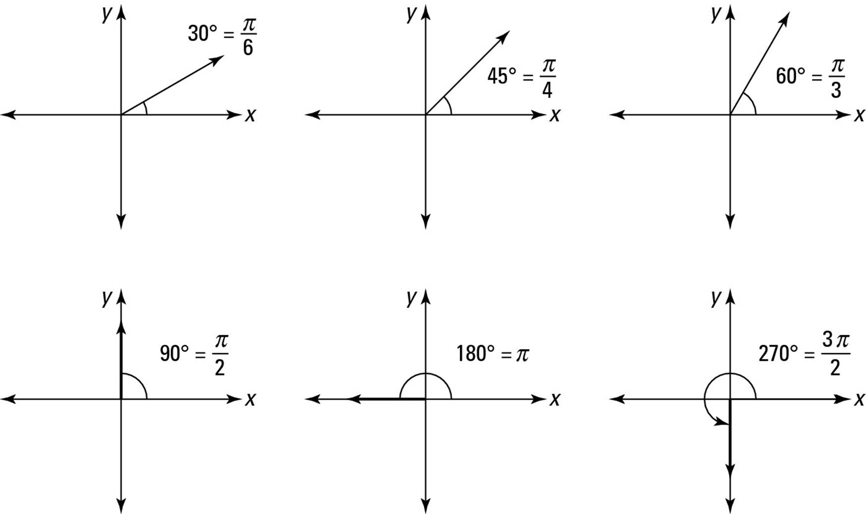
In any case, make sure you know the most common angles in both degrees and radians. Figure 2-2 shows you some common angles.

Radians are the basis of polar coordinates, which I discuss later in this section.

Graphing common functions

You should be familiar with how certain common functions look when drawn on a graph. In this section, I show you the most common graphs of functions. These functions are continuous, so they’re integrable at all real values of x.

Linear and polynomial functions

Figure 2-3 shows three simple linear functions.

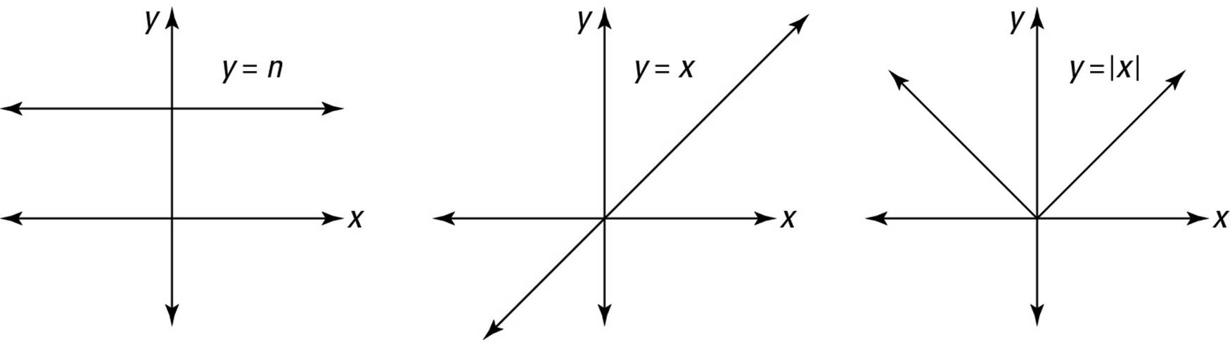
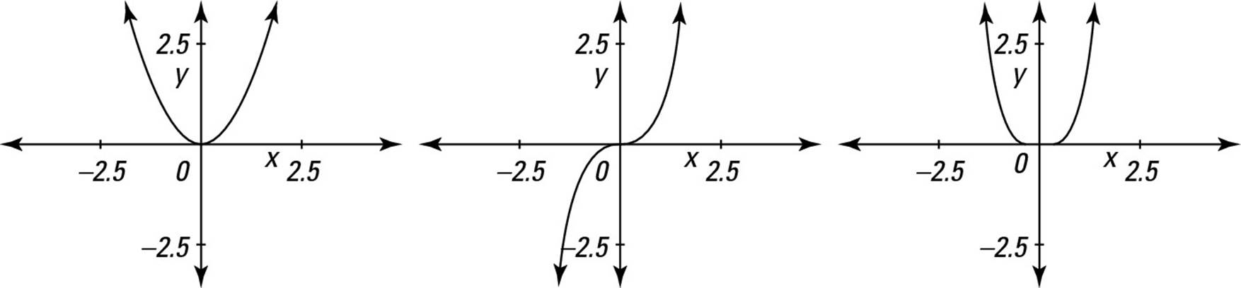
Figure 2-4 includes a few basic polynomial functions.

Exponential and logarithmic functions

Here are some exponential functions with whole number bases:

y = 2^x

y = 3^x

y = 10^x

Notice that for every positive base, the exponential function

Crosses the y-axis at y = 1

Explodes to infinity as x increases (that is, it has an unbounded y value)

Approaches y = 0 as x decreases (that is, in the negative direction the x-axis is an asymptote; you can read about these later)

The most important exponential function is e^x. See Figure 2-5 for a graph of this function.

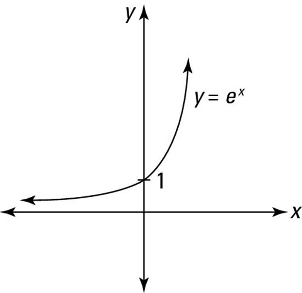
The unique feature of this exponential function is that at every value of x, its slope is e^x. That is, this function is its own derivative (see “Recent Memories: A Review of Calculus I” later in this chapter for more on derivatives).

Another important function is the logarithmic function (also called the natural log function). Figure 2-6 is a graph of the logarithmic function y = ln x.

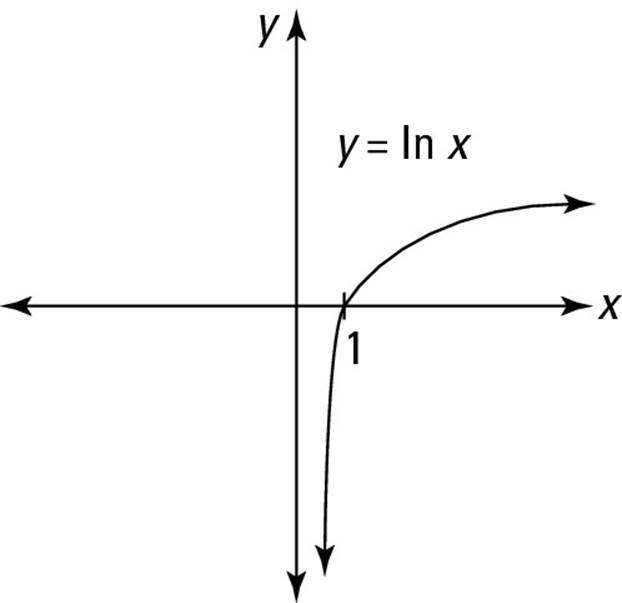
Notice that this function is the reflection of e^x along the diagonal line y = x. So the log function does the following:

Crosses the x-axis at x = 1

Explodes to infinity as x increases (that is, it has an unbounded y value), though more slowly than any exponential function

Produces a y value that approaches –∞ as x approaches 0 from the right

Furthermore, the domain of the log functions includes only positive values. That is, inputting a nonpositive value to the log function is a big no-no, on par with placing 0 in the denominator of a fraction or a negative value inside a square root.

For this reason, functions placed inside the log function often get “pretreated” with the absolute value operator. For example:

y = ln |x³|

You can bring an exponent outside of a natural log and make it a coefficient, as follows:

ln (a^b) = b ln a

Trigonometric functions

The two most important graphs of trig functions are the sine and cosine. See Figure 2-7 for graphs of these functions.

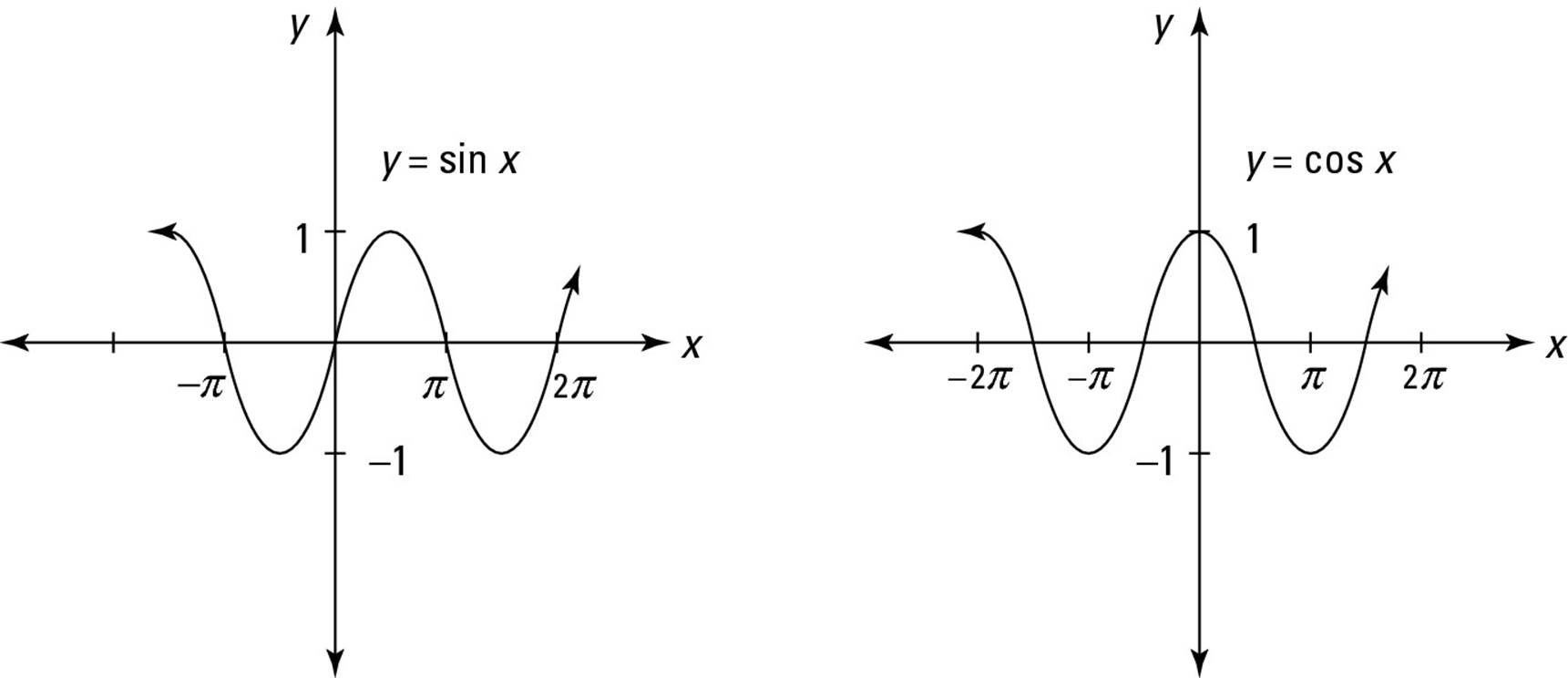
Note that the x values of these two graphs are typically marked off in multiples of π. Each of these functions has a period of 2π. In other words, it repeats its values after 2π units. And each has a maximum value of 1 and a minimum value of –1.

Remember that the sine function

Crosses the origin

Rises to a value of 1 at

Crosses the x-axis at all multiples of π

Remember that the cosine function

Has a value of 1 at x = 0

Drops to a value of 0 at

Crosses the x-axis at and so on

The graphs of other trig functions are also worth knowing. Figure 2-8 shows graphs of the trig functions y = tan x, y = cot x, y = sec x, and y = csc x.

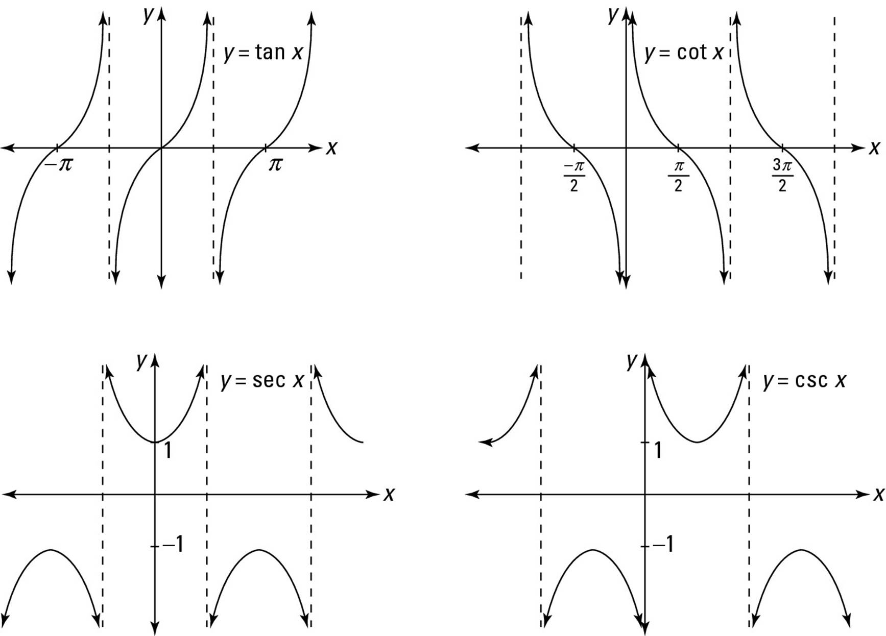
Asymptotes

An asymptote is any straight line on a graph that a curve approaches but doesn’t touch. It’s usually represented on a graph as a dashed line. For example, all four graphs in Figure 2-8 have vertical asymptotes.

Depending on the curve, an asymptote can run in any direction, including diagonally. When you’re working with functions, however, horizontal and vertical asymptotes are more common.

Transforming continuous functions

When you know how to graph the most common functions, you can transform them by using a few simple tricks, as I show you in Table 2-4.

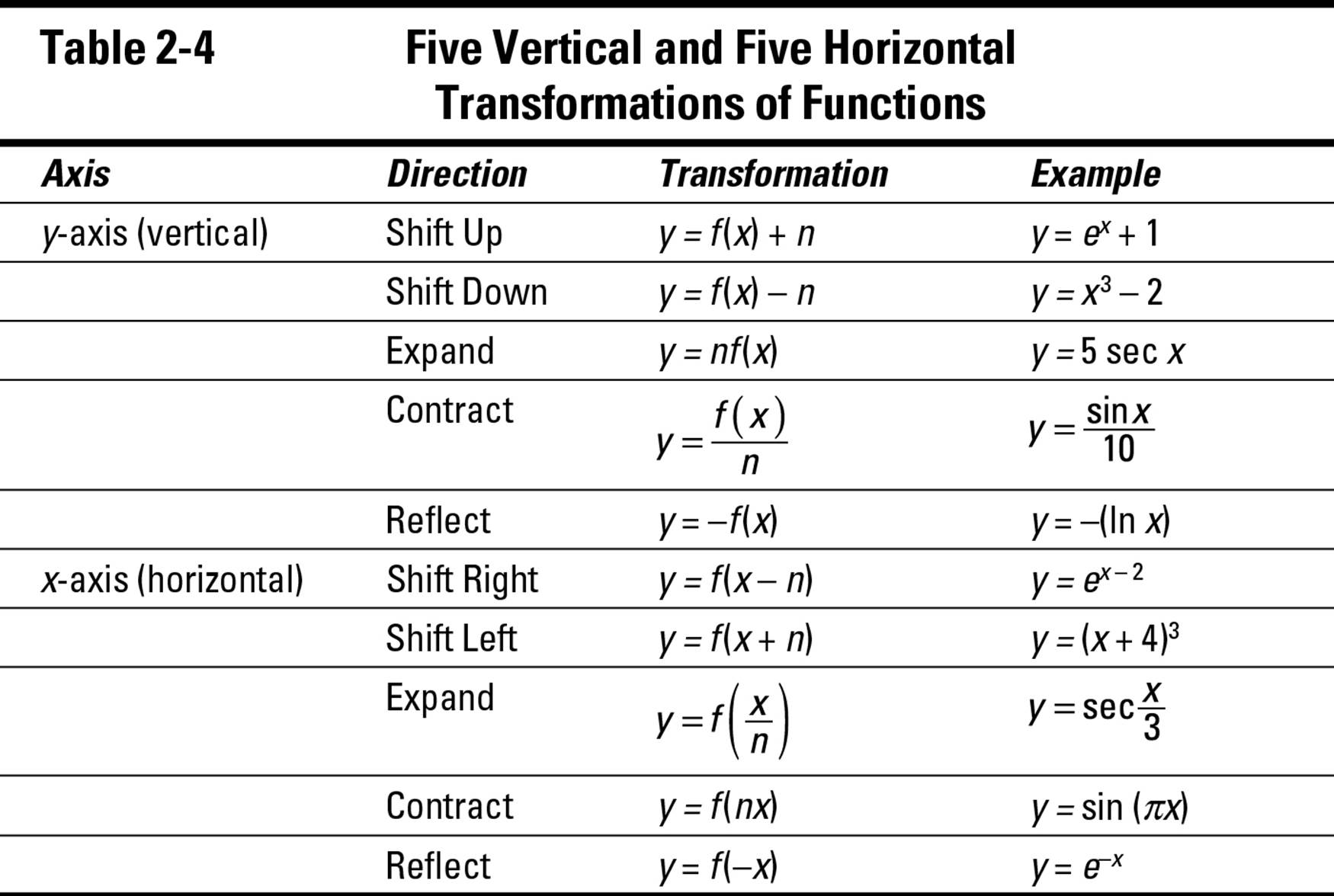
The vertical transformations are intuitive — that is, they take the function in the direction that you’d probably expect. For example, adding a constant shifts the function up and subtracting a constant shifts it down.

In contrast, the horizontal transformations are counterintuitive — that is, they take the function in the direction that you probably wouldn’t expect. For example, adding a constant shifts the function left and subtracting a constant shifts it right.

Identifying some important trig identities

I know that committing trig identities to memory registers on the Fun Meter someplace between alphabetizing your spice rack and vacuuming the lint filter on your dryer. But knowing a few important trig identities can be a lifesaver when you’re lost out on the misty calculus trails, so I recommend that you take a few along with you.

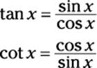
For starters, here are the three reciprocal identities, which you probably know already:

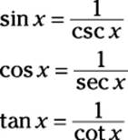
You also need these two important identities:

I call these the Basic Five trig identities. By using them, you can express any trig expression in terms of sines and cosines. Less obviously, you can also express any trig expression in terms of tangents and secants (try it!). Both of these facts are useful in Chapter 7, when I discuss trig integration.

Equally indispensable are the three square identities. Most students remember the first and forget about the other two, but you need to know them all:

sin² x + cos² x = 1

1 + tan² x = sec² x

1 + cot² x = csc² x

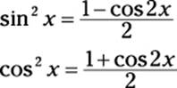
You also don’t want to be seen in public without the two half-angle identities:

Finally, you can’t live without the double-angle identities for sines:

sin 2x = 2 sin x cos x

Beyond these, if you have a little spare time, you can include these double-angle identities for cosines and tangents:

cos 2x = cos² x – sin² x = 2 cos² x – 1 = 1 – 2 sin² x

How to avoid an identity crisis

Most students remember the first square identity without trouble:

sin² x + cos² x = 1

If you’re worried you may forget the other two square identities just when you need them most, don’t despair. An easy way to remember them is to divide every term in the first square identity by cos² x to produce one new equation and by sin² x to produce another.

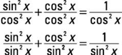
Now simplify these equations using the Basic Five trig identities:

1 + tan² x = sec² x

1 + cot² x = csc² x

Polar coordinates

Polar coordinates are an alternative to the Cartesian coordinate system. As with Cartesian coordinates, polar coordinates assign an ordered pair of values to every point on the plane. Unlike Cartesian coordinates, however, these values aren’t (x, y), but rather (r, θ).

The value r is the distance to the origin.

The value θ is the angular distance from the polar axis, which corresponds to the positive x-axis in Cartesian coordinates. (Angular distance is always measured counterclockwise.)

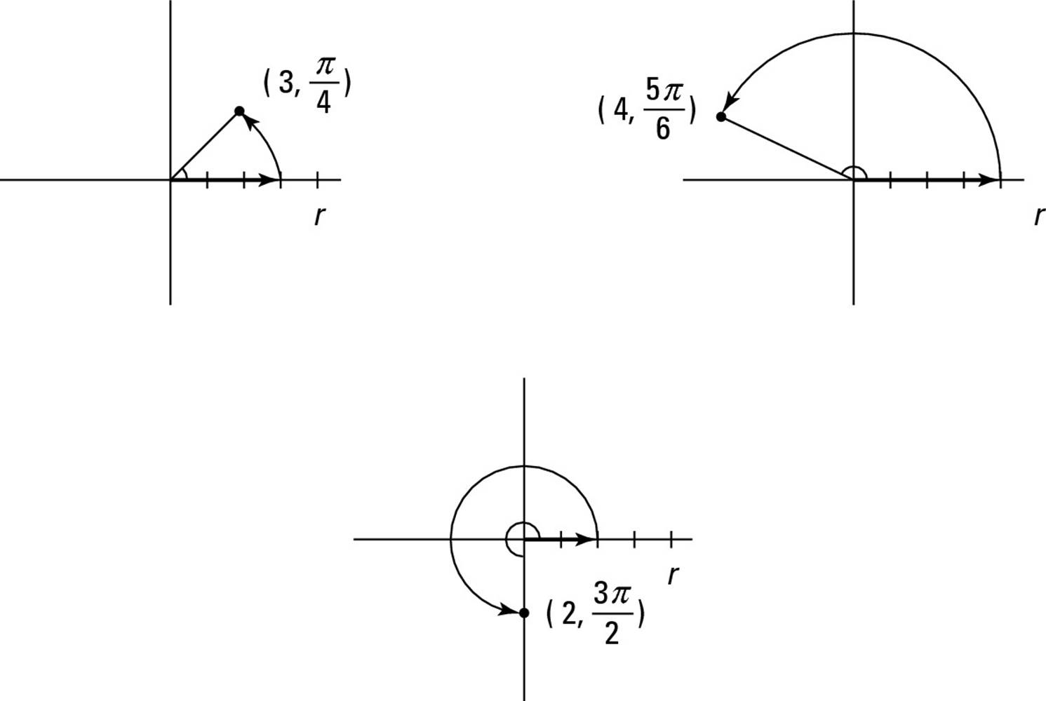
Figure 2-9 shows how to plot points in polar coordinates. For example:

To plot the point (3, ), travel 3 units from the origin on the polar axis, and then arc (equivalent to 45°) counterclockwise.

To plot (4, ), travel 4 units from the origin on the polar axis, and then arc units (equivalent to 150°) counterclockwise.

To plot the point (2, ), travel 2 units from the origin on the polar axis, and then arc units (equivalent to 270°) counterclockwise.

Polar coordinates allow you to plot certain shapes on the graph more simply than Cartesian coordinates. For example, here’s the equation for a 3-unit circle centered at the origin in both Cartesian and polar coordinates:

Some problems that would be difficult to solve expressed in terms of Cartesian variables (x and y) become much simpler when expressed in terms of polar variables (r and θ). To convert Cartesian variables to polar, use the following formulas:

x = r cos θ y = r sin θ

To convert polar variables to Cartesian, use these formulas:

Polar coordinates are the basis of two alternative 3-D coordinate systems: cylindrical coordinates and spherical coordinates. See Chapter 14 for a look at these two systems.

Summing up sigma notation

Mathematicians love sigma notation (Σ) for two reasons. First, it provides a convenient way to express a long or even infinite series. But even more important, it looks really cool and scary, which frightens nonmathematicians into revering mathematicians and paying them more money.

However, when you get right down to it, Σ is just fancy notation for adding, and even your little brother isn’t afraid of adding, so why should you be?

For example, suppose that you want to add the even numbers from 2 to 10. Of course, you can write this expression and its solution this way:

2 + 4 + 6 + 8 + 10 = 30

Or you can write the same expression by using sigma notation:

Here, n is the variable of summation — that is, the variable that you plug values into and then add. Below the Σ, you’re given the starting value of n (1) and above it the ending value (5). So here’s how to expand the notation:

You can also use sigma notation to stand for the sum of an infinite number of values — that is, an infinite series. For example, here’s how to add up all the positive square numbers:

This compact expression can be expanded as follows:

= 1² + 2² + 3² + 4² + ...

= 1 + 4 + 9 + 16 + ...

This sum is, of course, infinite. But not all infinite series behave in this way. In some cases, an infinite series equals a number. For example:

This series expands and evaluates as follows:

When a series evaluates to a number, the series is convergent. When a series isn’t convergent, it’s divergent. You find out all about divergent and convergent series in Chapter 12.

Recent Memories: A Review of Calculus I

Simply stated, integration is the study of how to solve a single problem — the area problem. Similarly, differentiation, which is the focus of Calculus I, is the study of how to solve the tangent problem: how to find the slope of the tangent line at any point on a curve. In this section, I review the highlights of Calculus I. For a more thorough review, see Calculus For Dummies by Mark Ryan (Wiley).

Knowing your limits

An important thread that runs through Calculus I is the concept of a limit. Limits are also important in Calculus II. In this section, I give you a review of everything you need to remember but may have forgotten about limits.

Telling functions and limits apart

A function provides a link between two variables: the independent variable (usually x) and the dependent variable (usually y). A function tells you the value y when x takes on a specific value. For example, here’s a function:

y = x²

In this case, when x takes a value of 2, the value of y is 4.

In contrast, a limit tells you what happens to y as x approaches a certain number without actually reaching it. For example, suppose that you’re working with the function y = x² and want to know the limit of this function as xapproaches 2. The notation to express this idea is as follows:

You can get a sense of what this limit equals by plugging successively closer approximations of 2 into the function (see Table 2-5).

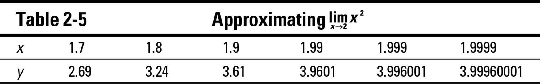
This table provides strong evidence that the limit evaluates to 4. That is:

Remember that this limit tells you nothing about what the function actually equals when x = 2. It tells you only that as x approaches 2, the value of the function gets closer and closer to 2. In this case, because the function and the limit are equal, the function is continuous at this point.

Evaluating limits

Evaluating a limit means either finding the value of the limit or showing that the limit doesn’t exist.

You can evaluate many limits by replacing the limit variable with the number that it approaches. For example:

Sometimes this replacement shows you that a limit doesn’t exist. For example:

When you find that a limit appears to equal either ∞ or –∞, the limit does not exist (DNE). DNE is a perfectly good way to complete the evaluation of a limit.

Some replacements lead to apparently untenable situations, such as division by zero. For example:

This looks like a dead end, because division by zero is undefined. But, in fact, you can actually get an answer to this problem. Remember that this limit tells you nothing about what happens when x actually equals 0, only what happens as x approaches 0: The denominator shrinks toward 0, while the numerator never falls below 1, so the value fraction becomes indefinitely large. Therefore:

Here’s another example:

This is another apparent dead end, because ∞ isn’t really a number, so how can it be the denominator of a fraction? Again, the limit saves the day. It doesn’t tell you what happens when x actually equals ∞ (if such a thing were possible), only what happens as x approaches ∞. In this case, the denominator becomes indefinitely large while the numerator remains constant. So

Some limits are more difficult to evaluate because they’re one of several indeterminate forms. The best way to solve them is to use L’Hopital’s Rule, which I discuss in detail at the end of this chapter.

Hitting the slopes with derivatives

The derivative at a given point on a function is the slope of the tangent line to that function at that point. The derivative of a function provides a “slope map” of that function.

The best way to compare a function with its derivative is by lining them up vertically. (See Figure 2-10 for an example.)

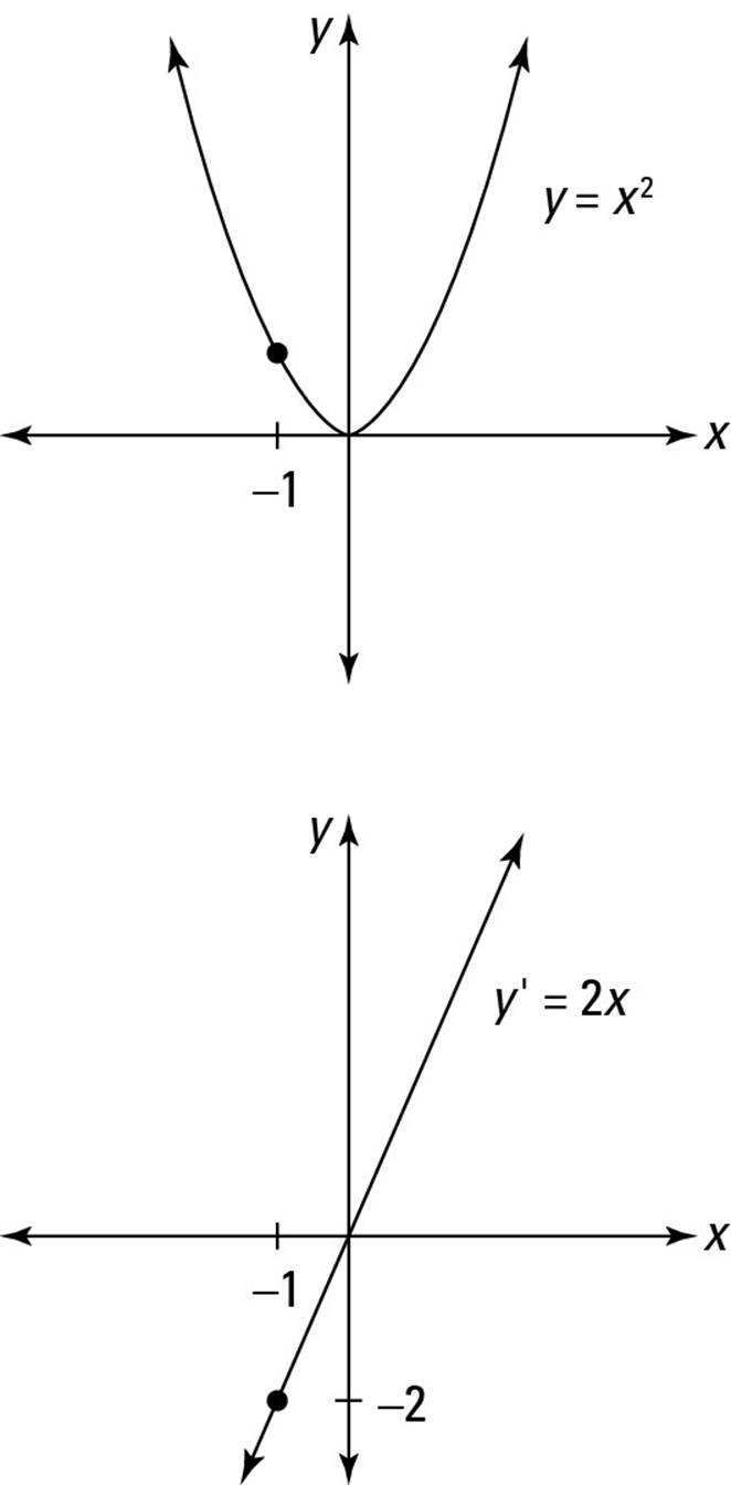
Looking at the top graph, you can see that when x = 0, the slope of the function y = x² is 0. The bottom graph verifies this because at x = 0, the derivative function y = 2x is also 0.

You probably can’t tell, however, what the slope of the top graph is at x = –1. To find out, look at the bottom graph and notice that at x = –1, the derivative function equals –2, so –2 is also the slope of the top graph at this point. Similarly, the derivative function tells you the slope at every point on the original function.

Referring to the limit formula for derivatives

In Calculus I, you develop two formulas for the derivative of a function. These formulas are both based on limits, and they’re both equally valid:

You probably won’t need to refer to these formulas much as you study Calculus II. Still, please keep in mind that the official definition of a function’s derivative is always cast in terms of a limit.

For a more detailed look at how these formulas are developed, see Calculus For Dummies by Mark Ryan (Wiley).

Knowing two notations for derivatives

Students often find the notation for derivatives — especially Leibniz notation — confusing. To make things simple, think of this notation as a unary operator that works in a similar way to a minus sign.

A minus sign attaches to the front of an expression, changing the value of that expression to its negative. Evaluating the effect of this sign on the expression is called distribution, which produces a new but equivalent expression. For example:

–(x² + 4x – 5) = –x² – 4x + 5

Similarly, the notation attaches to the front of an expression, changing the value of that expression to its derivative. Evaluating the effect of this notation on the expression is called differentiation, which also produces a new but equivalent expression. For example:

The basic notation remains the same even when an expression is recast as a function. For example, given the function y = f(x) = x² + 4x – 5, here’s how you differentiate:

The notation , which means “the change in y as x changes,” was first used by Gottfried Leibniz, one of the two inventors of calculus (the other inventor was Isaac Newton). An advantage of Leibniz notation is that it explicitly tells you the variable over which you’re differentiating — in this case, x. When this information is easily understood in context, a shorter notation is also available:

y' = f'(x) = 2x + 4

You should be comfortable with both of these forms of notation. I use them interchangeably throughout this book.

Understanding differentiation

Differentiation — the calculation of derivatives — is the central topic of Calculus I and makes an encore appearance in Calculus II.

In this section, I give you a refresher on some of the key topics of differentiation. I include the 17 need-to-know derivatives in this chapter. And if you’re shaky on the Chain Rule, I offer a clear explanation that gets you up to speed.

Memorizing key derivatives

The derivative of any constant is always 0:

The derivative of the variable by which you’re differentiating (in most cases, x) is 1:

Here are three more derivatives that are important to remember:

You need to know each of these derivatives as you move on in your study of calculus.

Derivatives of the trig functions

The derivatives of the six trig functions are as follows:

You need to know all these by heart.

Derivatives of the inverse trig functions

Two notations are commonly used for inverse trig functions. One is the addition of ^–1 to the function: sin^–1, cos^–1, and so forth. The second is the addition of arc to the function: arcsin, arccos, and so forth. They both mean the same thing, but I prefer the arc notation, because it’s less likely to be mistaken for an exponent.

I know that asking you to memorize these functions seems like a cruel joke. But you really need them when you get to trig substitution in Chapter 7, so at least have a look-see:

Notice that derivatives of the three “co” functions are just negations of the three other functions, so your work is cut in half.

The Sum Rule

In textbooks, the Sum Rule is often phrased like this: The derivative of the sum of functions equals the sum of the derivatives of those functions. Here’s the mathematical translation:

Simply put, the Sum Rule tells you that differentiating long expressions term by term is okay. For example, suppose that you want to evaluate the following:

The expression that you’re differentiating has three terms, so by using the Sum Rule, you can break the expression into three separate derivatives and solve them separately:

Note that the Sum Rule also applies to expressions of more than two terms. It also applies regardless of whether the term is positive or negative. Some books call this variation the Difference Rule, but you get the idea.

The Constant Multiple Rule

A typical textbook gives you this sort of definition for the Constant Multiple Rule: The derivative of a constant multiplied by a function equals the product of that constant and the derivative of that function. Check out the mathematical translation:

In plain English, this rule tells you that moving a constant outside of a derivative before you differentiate is okay. For example:

To solve this, move the 5 outside the derivative, and then differentiate:

The Power Rule

The Power Rule tells you that to find the derivative of x raised to any power, bring down the exponent as the coefficient of x, and then subtract 1 from the exponent and use this as your new exponent. Here’s the general form:

Here are a few examples:

When the function that you’re differentiating already has a coefficient, multiply the exponent by this coefficient. For example:

The Power Rule also extends to negative exponents, which allows you to differentiate many fractions. For example:

It also extends to fractional exponents, which allows you to differentiate square roots and other roots:

The Product Rule

The derivative of the product of two functions f(x) and g(x) is equal to the derivative of f(x) multiplied by g(x) plus the derivative of g(x) multiplied by f(x). That is:

= f'(x) · g(x) + g'(x) · f(x)

Practice saying the Product Rule like this: “The derivative of the first function times the second plus the derivative of the second times the first.” This encapsulates the Product Rule and sets you up to remember the Quotient Rule (see the next section).

For example, suppose that you want to differentiate e^x sin x. Start by breaking the problem out as follows:

Now you can evaluate both derivatives without much confusion:

= e^x · sin x + cos x · e^x

You can clean this up a bit as follows:

= e^x (sin x + cos x)

The Quotient Rule

Here’s what the Quotient Rule looks like:

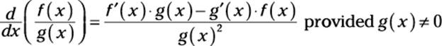
Practice saying the Quotient Rule like this: “The derivative of the top function times the bottom minus the derivative of the bottom times the top, over the bottom squared.” This is similar enough to the Product Rule that you can remember it.

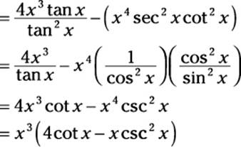
For example, suppose that you want to differentiate the following:

As you do with the Product Rule example in the preceding section, start by breaking the problem out as follows:

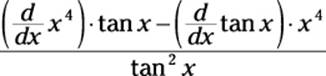
Now evaluate the two derivatives:

This answer is fine, but you can clean it up by using some algebra plus the Basic Five trig identities from earlier in this chapter. (Don’t worry too much about these steps unless your professor is particularly unforgiving.)

The Chain Rule

I’m aware that the Chain Rule is considered a major sticking point in Calculus I, so I want to take a little time to review it.

The Chain Rule allows you to differentiate nested functions — that is, functions within functions. It places no limit on how deeply nested these functions are. In this section, I show you an easy way to think about nested functions, and then I show you how to apply the Chain Rule simply.

Evaluating functions from the inside out

When you’re evaluating a nested function, you begin with the inner function and move outward. For example:

f(x) = e^2x

In this case, 2x is the inner function. To see why, suppose that you want to evaluate f(x) for a given value of x. To keep things simple, say that x = 0. After plugging in 0 for x, your first step is to evaluate the inner function, which I underline:

Step 1: e²⁽⁰⁾ = e⁰

Your next step is to evaluate the outer function:

Step 2: e⁰ = 1

The terms inner function and outer function are determined by the order in which the functions get evaluated. This is true no matter how deeply nested these functions are. For example:

Suppose that you want to evaluate g(x). To keep the numbers simple, this time let x = 2. After plugging in 2 for x, here’s the order of evaluation from the inner function to the outer:

Step 1:

Step 2:

Step 3:

Step 4: (ln 1)³ = 0³

Step 5: 0³ = 0

The process of evaluation clearly lays out the five nested functions of g(x) from inner to outer.

Differentiating functions from the outside in

In contrast to evaluation, differentiating a function using the Chain Rule forces you to begin with the outer function and move inward.

Here’s the basic Chain Rule the way that you find it in textbooks:

To differentiate nested functions using the Chain Rule, write down the derivative of the outer function, copying everything inside it, and multiply this result by the derivative of the next function inward.

This explanation may seem a bit confusing, but it’s a lot easier when you know how to find the outer function, which I explain in the previous section, “Evaluating functions from the inside out.” A couple of examples should help.

Suppose that you want to differentiate the nested function sin 2x. The outer function is the sine portion, so this is where you start:

To finish, you still need to differentiate 2x:

= cos 2x · 2

Rearranging this solution to make it more presentable gives you your final answer:

= 2 cos 2x

When you differentiate more than two nested functions, the Chain Rule really lives up to its name: As you break down the problem step by step, you string out a chain of multiplied expressions.

For example, suppose that you want to differentiate sin³ e^x. Remember from the earlier section, “Noting trig notation,” that the notation sin³ e^x really means (sin e^x)³. This rearrangement makes clear that the outer function is the power of 3, so begin differentiating with this function:

Now you have a smaller function, sin e^x, to differentiate:

Only one more derivative to go:

= 3(sin e^x)² · cos e^x · e^x

Again, rearranging your answer is customary:

= 3e^x cos e^x sin² e^x

Finding Limits Using L’Hopital’s Rule

L’Hopital’s Rule is all about limits and derivatives, so it fits better with Calculus I than Calculus II. But some colleges save this topic for Calculus II.

So even though I’m addressing this as a review topic, fear not: Here, I give you the full story of L’Hopital’s Rule, starting with how to pronounce L’Hopital (low-pee-tahl).

L’Hopital’s Rule provides a method for evaluating certain indeterminate forms of limits. First, I show you what an indeterminate form of a limit looks like, with a list of all common indeterminate forms. Next, I show you how to use L’Hopital’s Rule to evaluate some of these forms. And finally, I show you how to work with the other indeterminate forms so that you can evaluate them.

Understanding determinate and indeterminate forms of limits

As you discover earlier in this chapter, in “Knowing your limits,” you can evaluate many limits by simply replacing the limit variable with the number that it approaches. In some cases, this replacement results in a number, so this number is the value of the limit that you’re seeking. In other cases, this replacement gives you an infinite value (either +∞ or –∞), so the limit does not exist (DNE).

Table 2-6 shows a list of some functions that often cause confusion.

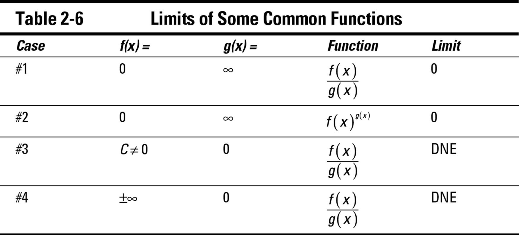
To understand how to think about these four cases, remember that a limit describes the behavior of a function very close to, but not exactly at, a value of x.

In the first and second cases, f(x) gets very close to 0 and g(x) explodes to infinity, so both and f(x)g⁽x⁾ approach 0. In the third case, f(x) is a constant C other than 0 and g(x) approaches 0, so the fraction explodes to infinity. And in the fourth case, f(x) explodes to infinity and g(x) approaches 0, so the fraction explodes to infinity.

In each of these cases, you have the answer you’re looking for — that is, you know whether the limit exists and, if so, its value — so these are all called determinate forms of a limit.

In contrast, however, sometimes when you try to evaluate a limit by replacement, the result is an indeterminate form of a limit. Table 2-7 includes two common indeterminate forms.

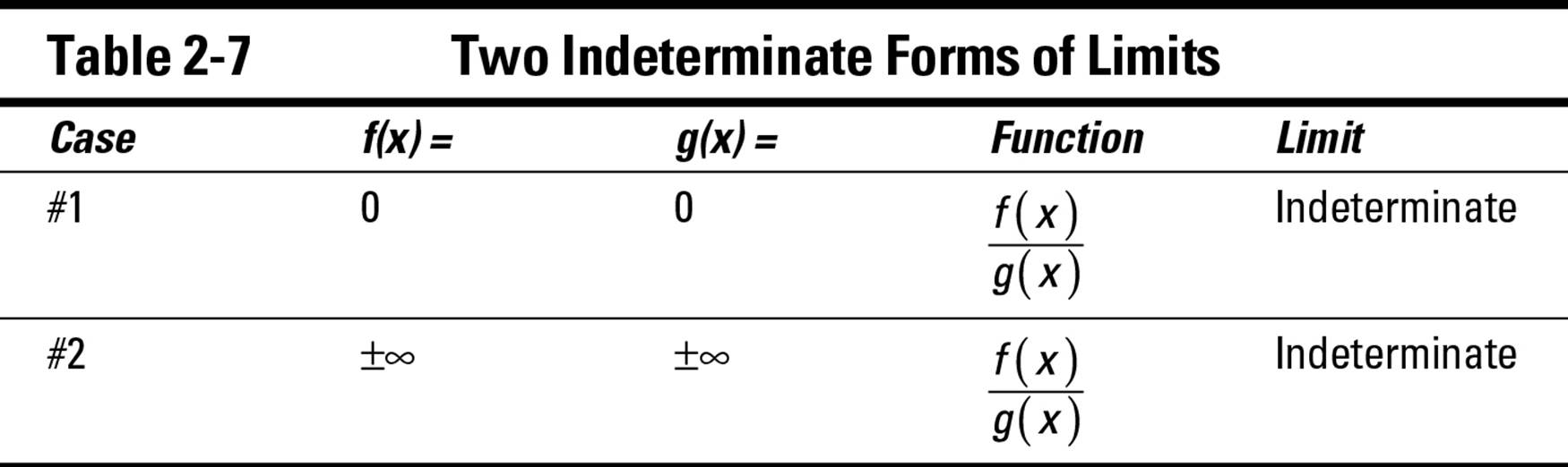
In these cases, the limit becomes a race between the numerator and denominator of the fractional function. For example, think about the second example in the chart. If f(x) crawls toward ∞ while g(x) zooms there, the fraction becomes bottom heavy and the limit is 0.

But if f(x) zooms to ∞ while g(x) crawls there, the fraction becomes top heavy and the limit is ∞ — that is, DNE. And if both functions move toward 0 proportionally, this proportion becomes the value of the limit.

When attempting to evaluate a limit by replacement saddles you with either of these forms, you need to do more work. Applying L’Hopital’s Rule is the most reliable way to get the answer that you’re looking for.

Introducing L’Hopital’s Rule

Suppose that you’re attempting to evaluate the limit of a function of the form . When replacing the limit variable with the number that it approaches results in either or , L’Hopital’s Rule tells you that the following equation holds true:

Note that c can be any real number as well as ∞ or –∞.

As an example, suppose that you want to evaluate the following limit:

Replacing x with 0 in the function leads to the following result:

This is one of the two indeterminate forms that L’Hopital’s Rule applies to, so you can draw the following conclusion:

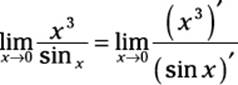
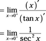
Next, evaluate the two derivatives:

Now use this new function to try another replacement of x with 0 and see what happens:

This time, the result is a determinate form, so you can evaluate the original limit as follows:

In some cases, you may need to apply L’Hopital’s Rule more than once to get an answer. For example:

Replacement of x with ∞ results in the indeterminate form , so you can use L’Hopital’s Rule:

In this case, the new function gives you the same indeterminate form, so use L’Hopital’s Rule again:

The same problem arises, but again you can use L’Hopital’s Rule. You can probably see where this example is going, so I fast-forward to the end:

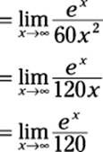
When you apply L’Hopital’s Rule repeatedly to a problem, make sure that every step along the way results in one of the two indeterminate forms that the rule applies to.

At last! The process finally yields a function with a determinate form:

Therefore, the limit doesn’t exist.

Alternative indeterminate forms

L’Hopital’s Rule applies only to the two indeterminate forms and .

But limits can result in a variety of other indeterminate forms for which L’Hopital’s Rule doesn’t hold. Table 2-8 is a list of the indeterminate forms that you’re most likely to see.

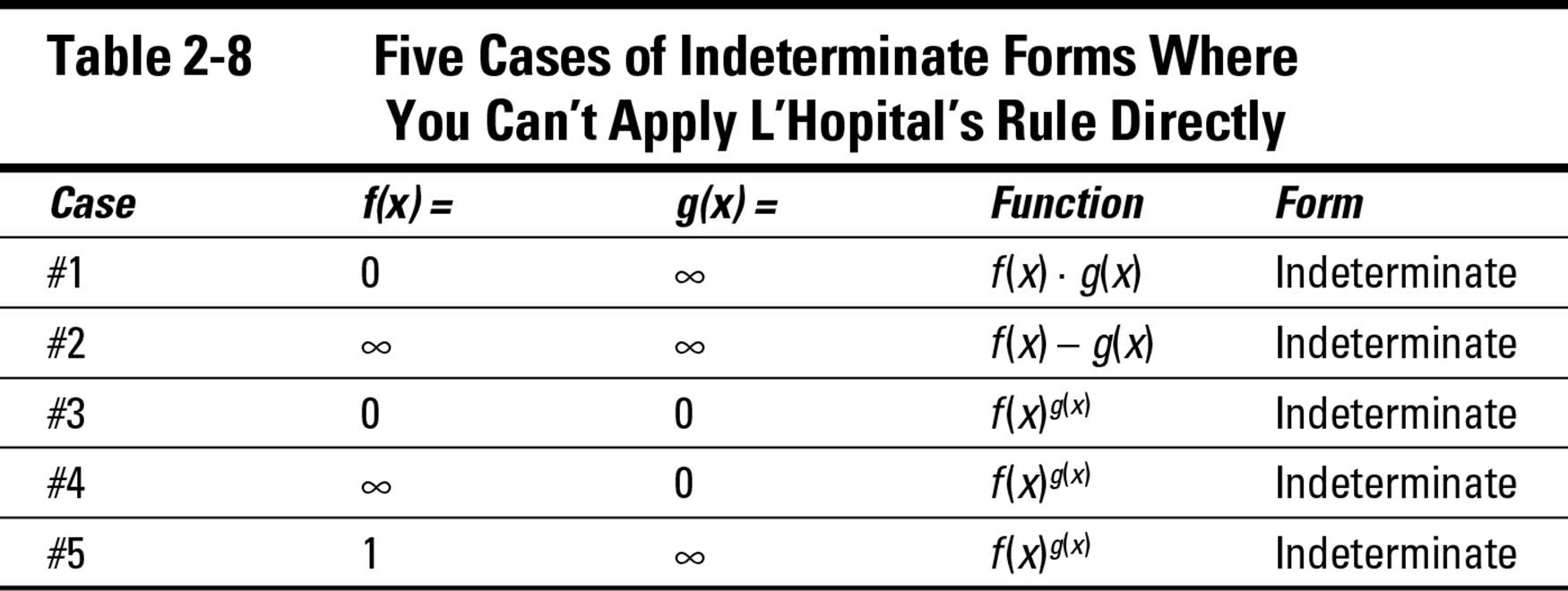
Because L’Hopital’s Rule doesn’t hold for these indeterminate forms, applying the rule directly gives you the wrong answer.

These indeterminate forms require special attention. In this section, I show you how to rewrite these functions so you can then apply L’Hopital’s Rule.

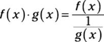
Case #1: 0 · ∞

When f(x) = 0 and g(x) = ∞, the limit of f(x) · g(x) is the indeterminate form 0 · ∞, which doesn’t allow you to use L’Hopital’s Rule. To evaluate this limit, rewrite this function as follows:

The limit of this new function is the indeterminate form , which allows you to use L’Hopital’s Rule. For example, suppose that you want to evaluate the following limit:

Replacing x with 0 gives you the indeterminate form 0 · ∞, so rewrite the limit as follows:

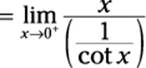
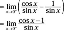
This can be simplified a little by using the inverse trig identity for cot x:

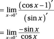
Now, replacing x with 0 gives you the indeterminate for , so you can apply L’Hopital’s Rule.

At this point, you can evaluate the limit directly by replacing x with 0:

Therefore, the limit evaluates to 1.

Case #2: ∞ – ∞

When f(x) = ∞ and g(x) = ∞, the limit of f(x) – g(x) is the indeterminate form ∞ – ∞, which doesn’t allow you to use L’Hopital’s Rule. To evaluate this limit, try to find a common denominator that turns the subtraction into a fraction. For example:

In this case, replacing x with 0 gives you the indeterminate form ∞ – ∞. A little tweaking with the Basic Five trig identities (see “Identifying some important trig identities” earlier in this chapter) does the trick:

Now, replacing x with 0 gives you the indeterminate form , so you can use L’Hopital’s Rule:

At last, you can evaluate the limit by directly replacing x with 0.

Therefore, the limit evaluates to 0.

Cases #3, #4, and #5: 0°, ∞°, and 1∞

In the following three cases, the limit of f(x)^g(x) is an indeterminate form that doesn’t allow you to use L’Hopital’s Rule:

When f(x) = 0 and g(x) = 0

When f(x) = ∞ and g(x) = 0

When f(x) = 1 and g(x) = ∞

This indeterminate form 1∞ is easy to forget because it seems weird. After all, 1^x = 1 for every real number, so why should 1∞ be any different? In this case, infinity plays one of its many tricks on mathematics. You can find out more about some of these tricks in Chapter 16.

For example, suppose that you want to evaluate the following limit:

As it stands, this limit is of the indeterminate form 0⁰.

Fortunately, I can show you a trick to handle these three cases. As with so many things mathematical, mere mortals such as you and me probably wouldn’t discover this trick, short of being washed up on a desert island with nothing to do but solve math problems and eat coconuts. However, somebody did the hard work already. Remembering this recipe is a small price to pay:

1. Set the limit equal to y.

2. Take the natural log of both sides, and then do some log rolling:

Here are the two log rolling steps:

• First, roll the log inside the limit:

This step is valid because the limit of a log equals the log of a limit (I know, those words veritably roll off the tongue).

• Next, roll the exponent over the log:

This step is also valid, as I show you earlier in this chapter when I discuss the log function in “Graphing common functions.”

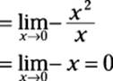
3. Evaluate this limit as I show you in “Case #1: 0 · ∞.”

Begin by changing the limit to a determinate form:

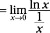
At last, you can apply L’Hopital’s Rule:

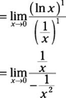
Now evaluating the limit isn’t too bad:

Wait! Remember that way back in Step 2 you set this limit equal to ln y. So you have one more step!

4. Solve for y.

Yes, this is your final answer, so .

This recipe works with all three indeterminate forms that I talk about at the beginning of this section. Just make sure that you keep tweaking the limit until you have one of the two forms that are compatible with L’Hopital’s Rule.