Calculus II For Dummies, 2nd Edition (2012)
Part I. Introduction to Integration
Chapter 3. From Definite to Indefinite: The Indefinite Integral
In This Chapter
![]() Approximating area in five different ways
Approximating area in five different ways
![]() Calculating sums and definite integrals
Calculating sums and definite integrals
![]() Looking at the Fundamental Theorem of Calculus (FTC)
Looking at the Fundamental Theorem of Calculus (FTC)
![]() Seeing how the indefinite integral is the inverse of the derivative
Seeing how the indefinite integral is the inverse of the derivative
![]() Clarifying the differences between definite and indefinite integrals
Clarifying the differences between definite and indefinite integrals
The first step to solving an area problem — that is, finding the area of a complex or unusual shape on the graph — is expressing it as a definite integral. In turn, you can evaluate a definite integral by using a formula based on the limit of a Riemann sum (as I show you in Chapter 1).
In this chapter, you get down to business calculating definite integrals. First, I show you a variety of different ways to estimate area. All these methods lead to a better understanding of the Riemann sum formula for the definite integral. Next, you use this formula to find exact areas. This rather hairy method of calculating definite integrals prompts a search for a better way.
This better way is the indefinite integral. I show you how the indefinite integral provides a much simpler way to calculate area. Furthermore, you find a surprising link between differentiation (which is the focus of Calculus I) and integration. This link, called the Fundamental Theorem of Calculus, shows that the indefinite integral is really an anti-derivative (the inverse of the derivative).
To finish up, I show you how using an indefinite integral to evaluate a definite integral results in signed area. I also clarify the differences between definite and indefinite integrals so that you never get them confused. By the end of this chapter, you’re ready for Part II, which focuses on an abundance of methods for calculating the indefinite integral.
Approximate Integration
Finding the exact area under a curve — that is, solving an area problem (see Chapter 1) — is one of the main reasons that integration was invented. But you can approximate area by using a variety of methods. Approximating area is a good first step toward understanding how integration works.
In this section, I show you five different methods for approximating the solution to an area problem. Generally speaking, I introduce these methods in the order of increasing difficulty and effectiveness. The first three involve manipulating rectangles.
![]() The first two methods — using left and right rectangles — are the easiest to use, but they usually give you the greatest margin of error.
The first two methods — using left and right rectangles — are the easiest to use, but they usually give you the greatest margin of error.
![]() The Midpoint Rule (slicing rectangles) is a little more difficult, but it usually gives you a slightly better estimate.
The Midpoint Rule (slicing rectangles) is a little more difficult, but it usually gives you a slightly better estimate.
![]() The Trapezoid Rule requires more computation, but it gives an even better estimate.
The Trapezoid Rule requires more computation, but it gives an even better estimate.
![]() Simpson’s Rule is the most difficult to grasp, but it gives the best approximation and, in some cases, provides you with an exact measurement of area.
Simpson’s Rule is the most difficult to grasp, but it gives the best approximation and, in some cases, provides you with an exact measurement of area.
Three ways to approximate area with rectangles
Slicing an irregular shape into rectangles is the most common approach to approximating its area (see Chapter 1 for more details on this approach). In this section, I show you three different techniques for approximating area with rectangles.
Using left rectangles
You can use left rectangles to approximate the solution to an area problem (see Chapter 1). For example, suppose that you want to approximate the shaded area in Figure 3-1 by using four left rectangles.
To draw these four rectangles, start by dropping a vertical line from the function to the x-axis at the left-hand limit of integration — that is, x = 0. Then drop three more vertical lines from the function to the x-axis at x = 2, 4, and 6. Next, at the four points where these lines cross the function, draw horizontal lines from left to right to make the top edges of the four rectangles. The left and top edges define the size and shape of each left rectangle.
Figure 3-1:Approximating![]() by using four left rectangles.
by using four left rectangles.
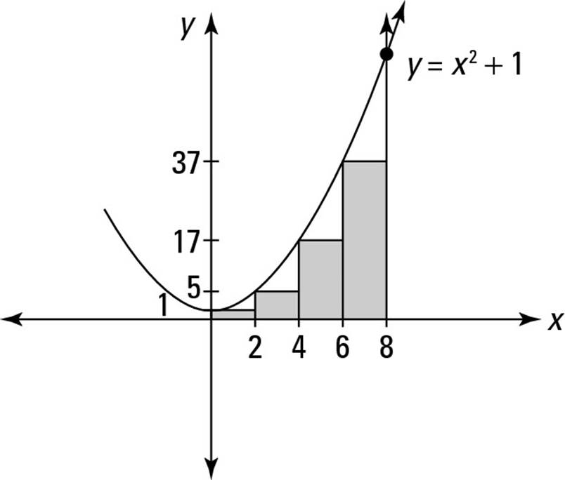
To measure the areas of these four rectangles, you need the width and height of each. The width of each rectangle is obviously 2. The height and area of each is determined by the value of the function at its left edge, as shown in Table 3-1.
To approximate the shaded area, add up the areas of these four rectangles:
Using right rectangles
Using right rectangles to approximate the solution to an area problem is virtually the same as using left rectangles. For example, suppose that you want to use six right rectangles to approximate the shaded area in Figure 3-2.
To draw these rectangles, start by dropping a vertical line from the function to the x-axis at the right-hand limit of integration — that is, x = 3. Next, drop five more vertical lines from the function to the x-axis at x = 0.5, 1, 1.5, 2, and 2.5. Then, at the six points where these lines cross the function, draw horizontal lines from right to left to make the top edges of the six rectangles. The right and top edges define the size and shape of each right rectangle.
Figure 3-2:Approximating ![]() by using six right rectangles.
by using six right rectangles.
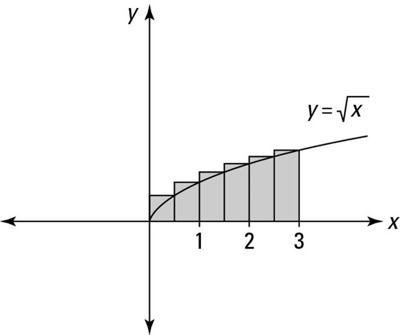
To measure the areas of these six rectangles, you need the width and height of each. Each rectangle’s width is 0.5. Its height and area are determined by the value of the function at its right edge, as shown in Table 3-2.
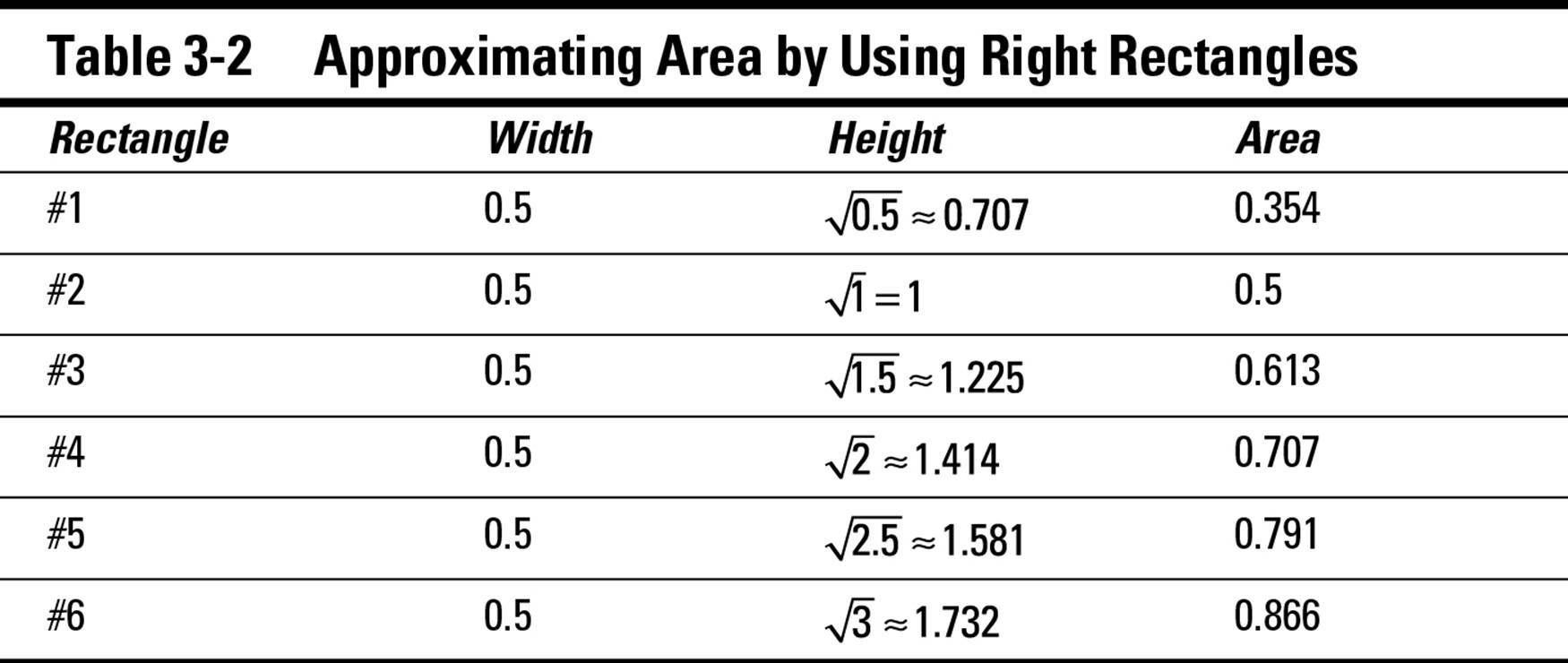
To approximate the shaded area, add up the areas of these six rectangles:
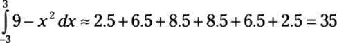
Finding a middle ground: The Midpoint Rule
Both left and right rectangles give you a decent approximation of area. So it stands to reason that slicing an area vertically and measuring the height of each rectangle from the midpoint of each slice might give you a slightly better approximation of area.
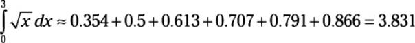
For example, suppose that you want to use midpoint rectangles to approximate the shaded area in Figure 3-3.
Figure 3-3:Approximating![]() by using three midpoint rectangles.
by using three midpoint rectangles.
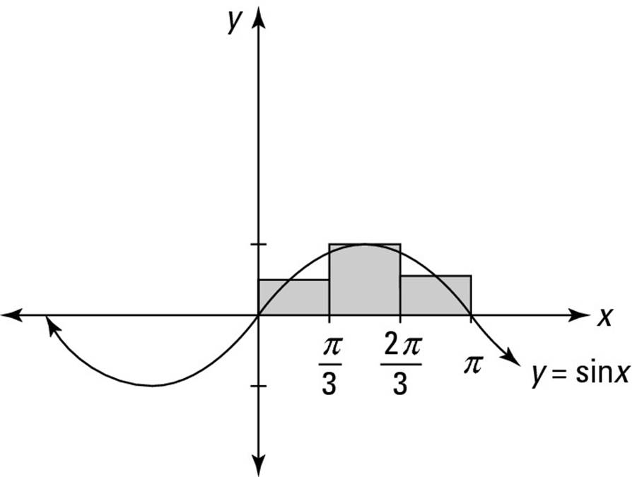
To draw these three rectangles, start by drawing vertical lines that intersect both the function and the x-axis at x = 0, ![]() ,
, ![]() , and π. Next, find where the midpoints of these three regions — that is,
, and π. Next, find where the midpoints of these three regions — that is, ![]() ,
, ![]() , and
, and ![]() — intersect the function. Now draw horizontal lines through these three points to make the tops of the three rectangles.
— intersect the function. Now draw horizontal lines through these three points to make the tops of the three rectangles.
To measure these three rectangles, you need the width and height of each to compute the area. The width of each rectangle is ![]() , and the height is given in Table 3-3.
, and the height is given in Table 3-3.
To approximate the shaded area, add up the areas of the three rectangles:
![]()
The slack factor
The formula for the definite integral is based on Riemann sums (see Chapter 1). This formula allows you to add up the area of infinitely many rectangular slices that are infinitesimally thin to find the exact solution to an area problem.
And here’s the strange part: Within certain parameters, the Riemann sum formula doesn’t care how you do the slicing. All three slicing methods that I discuss earlier work equally well. That is, although each method yields a different approximate area for a given finite number of slices, all these differences are smoothed over when the limit is applied. In other words, all three methods work to provide you the exact area for infinitely many slices.
I call this feature of measuring rectangles the slack factor. Understanding the slack factor helps you understand why using rectangles drawn at the left endpoint, right endpoint, or midpoint all lead to the same exact value of an area: As you measure progressively thinner slices, the slack factor never increases and tends to decrease. As the number of slices approaches ∞, the width of each slice approaches 0, so the slack factor also approaches 0.
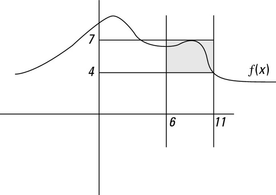
Figure 3-4 shows the range of this slack in choosing a rectangle. In this example, to find the area under f(x), you need to measure a rectangle inside the given slice (between 6 and 11). The height of this rectangle must be inclusively between 4 and 7, the local maximum and minimum of f(x). Within these parameters, however, you can measure any rectangle. So this particular slice has a width of 5 (because 11 – 6 = 5), but it can have any height from 4 to 7. Therefore, the resulting area of this slice can be any value from 20 (because 5 · 4 = 20) to 35 (because 5 · 7 = 35).
The slack factor explains why a variety of ways of measuring the size of rectangles — including the Trapezoid Rule and Simpson’s Rule (see the next section) — are all acceptable when calculating the Riemann sum.
Figure 3-4: For each slice you’re measuring, you can use any rectangle that passes through the function at one point or more.
Two more ways to approximate area
Although slicing a region into rectangles is the simplest way to approximate its area, rectangles aren’t the only shape that you can use. For finding many areas, other shapes can yield a better approximation in fewer slices.
In this section, I show you two common alternatives to rectangular slicing: the Trapezoid Rule (which, not surprisingly, uses trapezoids) and Simpson’s Rule (which uses rectangles topped with parabolas).
Feeling trapped? The Trapezoid Rule
In case you feel restricted — dare I say boxed in? — by estimating areas with only rectangles, you can get an even closer approximation by drawing trapezoids instead of rectangles.
For example, suppose that you want to use six trapezoids to estimate this area:
You can probably tell just by looking at the graph in Figure 3-5 that using trapezoids gives you a closer approximation than rectangles. In fact, the area of a trapezoid drawn on any slice of a function will be the average of the areas of the left and right rectangles drawn on that slice.
Figure 3-5:Approximating ![]() by using six trapezoids.
by using six trapezoids.
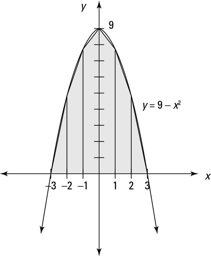
To draw these six trapezoids, first plot points along the function at x = –3, –2, –1, 0, 1, 2, and 3. Next, connect adjacent points to make the top edges of the trapezoids. Finally, draw vertical lines through these points.
 Two of the six “trapezoids” are actually triangles. This fact doesn’t affect the calculation; just think of each triangle as a trapezoid with one height equal to zero.
To find the area of these six trapezoids, use the formula for the area of a trapezoid that you know from geometry: ![]() . In this case, however, the two bases — that is, the parallel sides of the trapezoid — are the heights on the left and right sides. As always, the width is easy to calculate — in this case, it’s 1. Table 3-4 shows the rest of the information for calculating the area of each trapezoid.
. In this case, however, the two bases — that is, the parallel sides of the trapezoid — are the heights on the left and right sides. As always, the width is easy to calculate — in this case, it’s 1. Table 3-4 shows the rest of the information for calculating the area of each trapezoid.
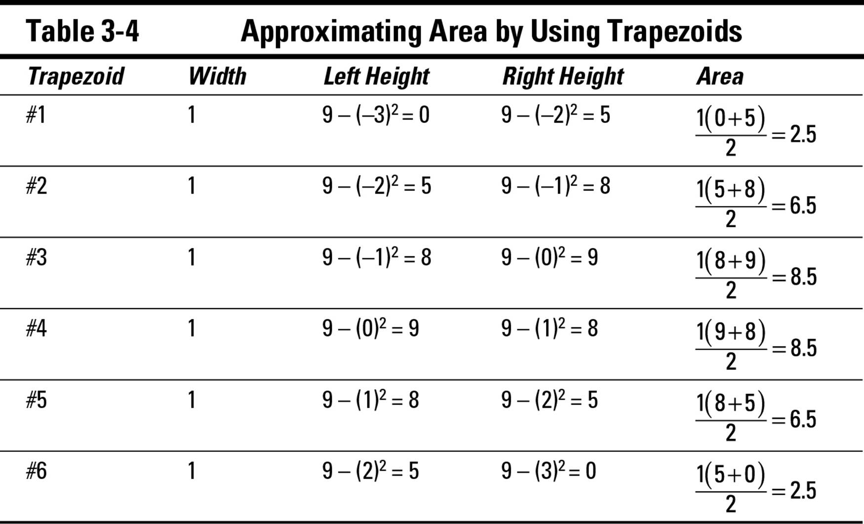
To approximate the shaded area, find the sum of the six areas of the trapezoids:
Don’t have a cow! Simpson’s Rule
You may recall from geometry that you can draw exactly one circle through any three nonlinear points. You may not recall, however, that the same is true of parabolas: Just three nonlinear points determine a parabola.
Simpson’s Rule relies on this geometric theorem. When using Simpson’s Rule, you use left and right endpoints as well as midpoints as these three points for each slice.
1. Begin slicing the area that you want to approximate into strips that intersect the function.
2. Mark the left endpoint, midpoint, and right endpoint of each strip.
3. Top each strip with the section of the parabola that passes through these three points.
4. Add up the areas of these parabola-topped strips.
At first glance, Simpson’s Rule seems a bit circular: You’re trying to approximate the area under a curve, but this method forces you to measure the area inside a region that includes a curve. Fortunately, Thomas Simpson, who invented this rule, is way ahead on this one. His method allows you to measure these strangely shaped regions without too much difficulty.
Without further ado, here’s Simpson’s Rule:
Given that n is an even number,
![]()
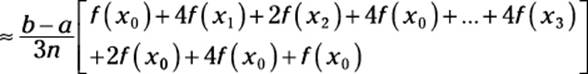
What does it all mean? As with every approximation method you’ve encountered, the key to Simpson’s Rule is measuring the width and height of each of these regions (with some adjustments):
![]() The width is represented by
The width is represented by ![]() — but Simpson’s Rule adjusts this value to
— but Simpson’s Rule adjusts this value to ![]() .
.
![]() The heights are represented by f(x) taken at various values of x — but Simpson’s Rule multiplies some of these by a coefficient of either 4 or 2. (By the way, these choices of coefficients are based on the known result of the area under a parabola — not just picked out of the air!)
The heights are represented by f(x) taken at various values of x — but Simpson’s Rule multiplies some of these by a coefficient of either 4 or 2. (By the way, these choices of coefficients are based on the known result of the area under a parabola — not just picked out of the air!)
The best way to show you how this rule works is with an example. Suppose that you want to use Simpson’s Rule to approximate the following:

First, divide the area that you want to approximate into an even number of regions — say, eight — by drawing nine vertical lines from x = 1 to x = 5. Now top these regions off with parabolas as I show you in Figure 3-6.
Figure 3-6:Approximating![]() by using Simpson’s Rule.
by using Simpson’s Rule.
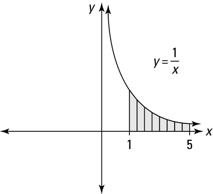
The width of each region is 0.5, so adjust this by dividing by 3:
![]()
Moving on to the heights, find f(x) when x = 1, 1.5, 2, ... , 4.5, and 5 (see the second column of Table 3-5). Adjust all these values except the first and the last by multiplying by 4 or 2, alternately.
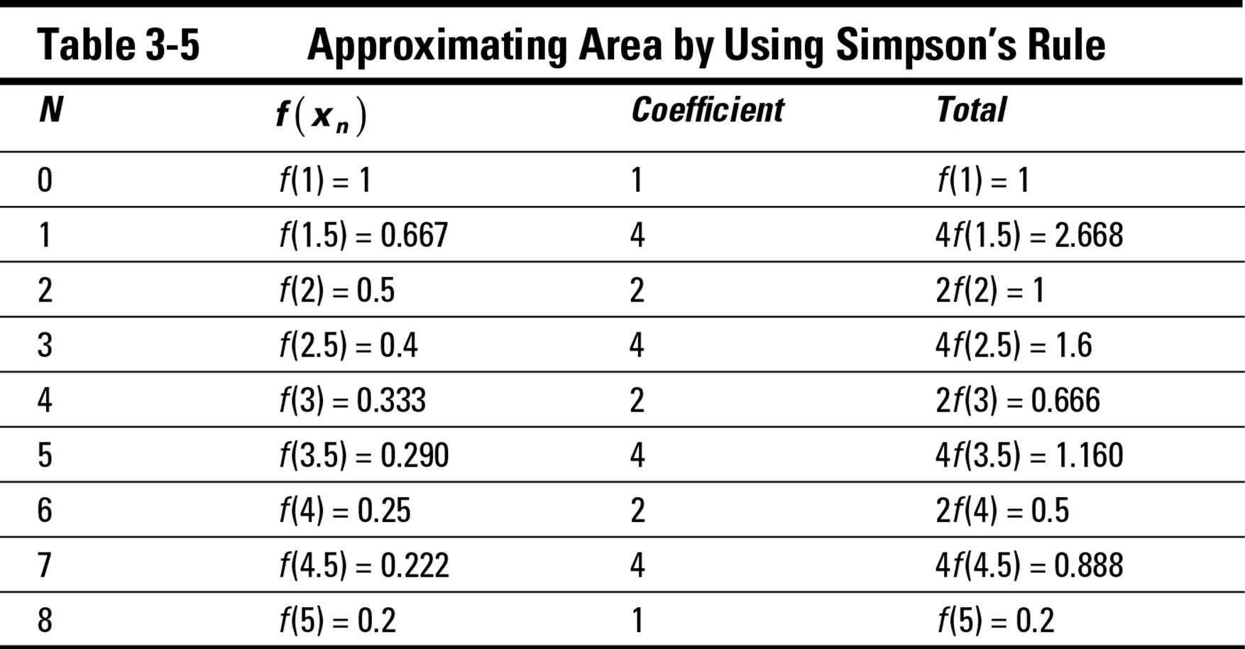
Now apply Simpson’s Rule as follows:
≈ 0.167 (1 + 2.668 + 1 + 1.6 + 0.666 + 1.16 + 0.5 + 0.888 + 0.2)
= 0.167 (9.682) ≈ 1.617
So Simpson’s Rule approximates the area of the shaded region in Figure 3-6 as 1.617. (By the way, the actual area to three decimal places is about 1.609 — so Simpson’s Rule provides a pretty good estimate.)
 In fact, Simpson’s Rule often provides an even better estimate than this example leads you to believe, because a lot of inaccuracy arises from rounding off decimals. In this case, when you perform the calculations with enough precision, Simpson’s Rule provides the correct area to three decimal places!
Knowing Sum-Thing about Summation Formulas
In Chapter 1, I introduce you to the Riemann sum formula for the definite integral. This formula includes a summation using sigma notation (Σ). (Please flip to Chapter 2 if you need a refresher on this topic.)
In practice, evaluating a summation can be a little tricky. Fortunately, three important summation formulas exist to help you. In this section, I introduce you to these formulas and show you how to use them. In the next section, I show you how and when to apply them when you’re using the Riemann sum formula to solve an area problem.
The summation formula for counting numbers
The summation formula for counting numbers gives you an easy way to find the sum 1 + 2 + 3 + ... + n for any value of n:
![]()
To see how this formula works, suppose that n = 9:
![]()
The summation formula for counting numbers also produces this result:
![]()
According to a popular story, mathematician Karl Friedrich Gauss derived this formula as a schoolboy, when his teacher gave the class the boring task of adding up all the counting numbers from 1 to 100 so that he (the teacher) could nap at his desk. Within minutes, Gauss arrived at the correct answer, 5,050, disturbing his teacher’s snooze time and making mathematical history.
The summation formula for square numbers
The summation formula for square numbers gives you a quick way to add up 1 + 4 + 9 + ... + n2 for any value of n:
![]()
For example, suppose that n = 7:
![]()
The summation formula for square numbers gives you the same answer:
![]()
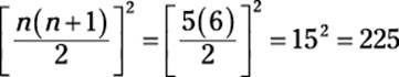
The summation formula for cubic numbers
The summation formula for cubic numbers gives you a quick way to add up 1 + 8 + 27 + ... + n3 for any value of n:
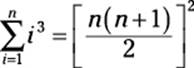
For example, suppose that n = 5:
![]()
The summation formula for cubic numbers produces the same result:
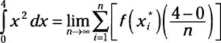
As Bad as It Gets: Calculating Definite Integrals Using the Riemann Sum Formula
In Chapter 1, I introduce you to this hairy equation for calculating the definite integral:
![]()
You may be wondering how practical this little gem is for calculating area. That’s a valid concern. The bad news is that this formula is, indeed, hairy and you need to understand how to use it to pass your first Calculus II exam.
But I have good news, too. In the beginning of Calculus I, you work with an equally hairy equation for calculating derivatives (see Chapter 2 for a refresher). Fortunately, later on, you find a bunch of easier ways to calculate derivatives.
This good news applies to integration, too. Later in this chapter, I show you how to make your life easier. In this section, however, I focus on how to use the Riemann sum formula to calculate the definite integral.
Before I get started, take another look at the Riemann sum formula and notice that the right side of this equation breaks down into four separate “chunks”:
![]() The limit:
The limit: ![]()
![]() The sum:
The sum: ![]()
![]() The function: f(x*i)
The function: f(x*i)
![]() The width (based on the limits of integration):
The width (based on the limits of integration): ![]()
To solve an integral using this formula, work backward, step by step, as follows:
1. Plug the limits of integration into the formula.
2. Rewrite the function f(x*i) as a summation in terms of i and n.
3. Calculate the sum.
4. Evaluate the limit.
Plugging in the limits of integration
In this section, I show you how to calculate the following integral:

This step is a no-brainer: You just plug the limits of integration — that is, the values of a and b — into the formula:
Before moving on, I know that you just can’t go on living until you simplify 4 – 0:
![]()
That’s it!
Expressing the function as a sum in terms of i and n
This is the tricky step. It’s more of an art than a science, so if you’re an art major who just happens to be taking a Calculus II course, this just might be your lucky day (or maybe not).
To start out, think about how you would estimate  by using right rectangles, as I explain earlier in this chapter. Table 3-6 shows you how to do this, using one, two, four, and eight rectangles.
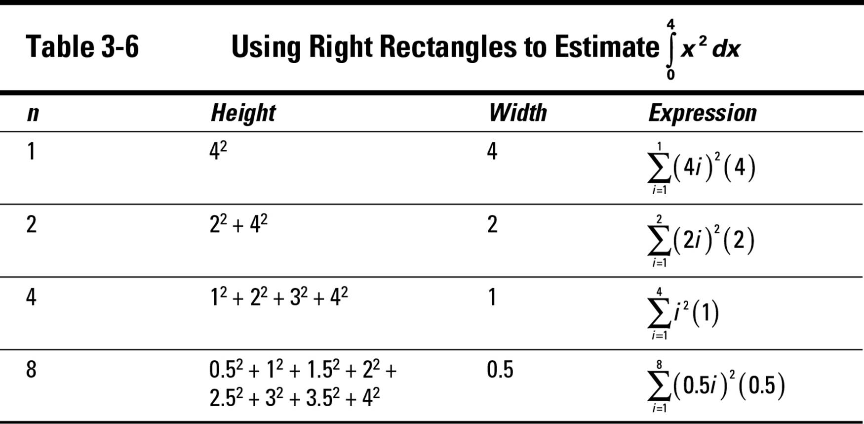
Your goal now is to find a general expression of the form ![]() that works for every value of n. In the preceding section, you find that
that works for every value of n. In the preceding section, you find that ![]() produces the correct width. In the last column of Table 3-6, I tease out this factor in each row — respectively, 4, 2, 1, and 0.5.
produces the correct width. In the last column of Table 3-6, I tease out this factor in each row — respectively, 4, 2, 1, and 0.5.
Now you need to find an expression in terms of the variable i that produces the height. In each row of Table 3-6, I show you the heights of the rectangles and the summation expression that produces these heights. So the question becomes, what single expression in terms of i and n produces
(4i)2 when n = 1
(2i)2 when n = 2
i2 when n = 4
(0.5i)2 when n = 16
The short answer is that the expression ![]() serves this purpose. For example, here’s what happens in the third row, when n = 4:
serves this purpose. For example, here’s what happens in the third row, when n = 4:
![]()
Thus, the part of the summation related to the height of the rectangles is evaluated as follows:
![]()
So here’s the general expression that you’re looking for:
![]()
Make sure that you understand why this expression works for all values of n before moving on. The first fraction represents the height of the rectangles and the second fraction represents the width, expressed as ![]() .
.
You can simplify this expression as follows:
![]()
Don’t forget before moving on that the entire expression is a limit as n approaches infinity:
![]()
 At this point in the problem, you have an expression that’s based on two variables: i and n. Remember that the two variables i and n are in the sum, and the variable x should already have exited.
Calculating the sum
Now you need a few tricks for calculating the summation portion of this expression:
![]()
You can move a constant outside of a summation without changing the value of that expression:
![]()
At this point, only the variables i and n are left inside the summation.
Remember that i stands for icky and n stands for nice. The variable n is nice because you can move it outside the summation just as if it were a constant:
![]()
Solving the problem with a summation formula
To handle the icky variable, i, you need a little help. Earlier in the chapter, in “Knowing Sum-Thing about Summation Formulas,” I give you some important formulas for handling this summation and others like it.
Getting back to the example, here’s where you left off:
![]()
To evaluate the sum ![]() , use the summation formula for square numbers:
, use the summation formula for square numbers:
![]()
A bit of algebra — which I omit because I know you can do it! — makes the problem look like this:
![]()
You’re now set up for the final — and easiest — step.
Evaluating the limit
At this point, the limit that you’ve probably been dreading all this time turns out to be the simplest part of the problem. As n approaches infinity, the two terms with n in the denominator approach 0, so they drop out entirely:
![]()
Yes, this is your final answer! Please note that because you used the Riemann sum formula, this is not an approximation, but the exact area under the curve y = x2 from 0 to 4.
Light at the End of the Tunnel: The Fundamental Theorem of Calculus
Finding the area under a curve — that is, solving an area problem — can be formalized using the definite integral (as you discover in Chapter 1). And the definite integral, in turn, is defined in terms of the Riemann sum formula. But, as you find out earlier in this chapter, the Riemann sum formula usually results in lengthy and difficult calculations.
There must be a better way! And, indeed, there is.
The Fundamental Theorem of Calculus (FTC) provides the link between derivatives and integrals. At first glance, these two ideas seem entirely unconnected, so the FTC seems like a bit of mathematical black magic. On closer examination, however, the connection between a function’s derivative (its slope) and its integral (the area underneath it) becomes clearer.
In this section, I show you the connection between slope and area. After you see this, the FTC will make more intuitive sense. At that point, I introduce the exact theorem and show you how to use it to evaluate integrals as anti-derivatives — that is, by understanding integration as the inverse of differentiation.
Without further ado, here’s the Fundamental Theorem of Calculus (FTC) in its most useful form:
If f'(x) is continuous on the closed interval [a, b],
![]()
The mainspring of this equality is the connection between f and its derivative function f'. To solve an integral, you need to be able to undo differentiation and find the original function f.
Many math books use the following notation for the FTC:
![]()
Both notations are equally valid, but I find this version a bit less intuitive than the version that I give you.
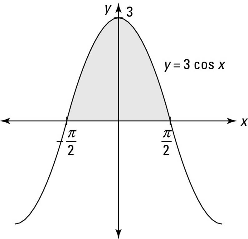
The FTC makes evaluating integrals a whole lot easier. For example, suppose that you want to evaluate the following:
![]()
This is the function that you see in Figure 3-3. The FTC allows you to solve this problem by thinking about it in a new way. First notice that the following statement is true:
f(x) = –cos x → f'(x) = sin x
So the FTC allows you to draw this conclusion:
![]()
Now you can solve this problem using simple trig:
= 1 + 1 = 2
So the exact (not approximate) shaded area in Figure 3-3 is 2 — all without drawing rectangles! The approximation using the Midpoint Rule (see “Finding a middle ground: The Midpoint Rule” earlier in this chapter) is 2.0944.
As another example, here’s the integral that, earlier in the chapter, you solved with the Riemann sum formula:
Begin by noticing that the following statement is true:
![]()
Now use the FTC to write this equation:
At this point, the solution becomes a matter of arithmetic:
![]()
In just three simple steps, the definite integral is solved without resorting to the hairy Riemann sum formula!
Understanding the Fundamental Theorem of Calculus
In the previous section, I show you just how useful the Fundamental Theorem of Calculus (FTC) can be for finding the exact value of a definite integral without using the Riemann sum formula. But why does the theorem work?
The FTC implies a connection between derivatives and integrals that isn’t intuitively obvious. In fact, the theorem implies that derivatives and integrals are inverse operations. It’s easy to see why other pairs of operations — such as addition and subtraction — are inverses. But how do you see this same connection between derivatives and integrals?
In this section, I give you a few ways to better understand this connection.
What’s slope got to do with it?
The idea that derivatives and integrals are connected — that is, the slope of a curve and the area under it are linked mathematically — seems odd until you spend some time thinking about it.
Solving a 200-year-old problem
The connection between derivatives and integrals as inverse operations was first noticed by Isaac Barrow (the teacher of Isaac Newton) in the 17th century. Newton and Gottfried Leibniz (the two key inventors of calculus) both made use of it as a conjecture — that is, as a mathematical statement that’s suspected to be true but hasn’t been proven yet.
But the FTC wasn’t officially proven in all its glory until your old friend Bernhard Riemann demonstrated it in the 19th century. During this 200-year lag, a lot of math — most notably, real analysis — had to be invented before Riemann could prove that derivatives and integrals are inverses.
If you have a head for business, here’s a practical way to understand the connection. Imagine that you run your own company. Envision a graph with a line as your net income (money coming in) and the area under the graph as your net savings (money in the bank). To keep this simple, imagine for the moment that this is a happy world where you have no expenses draining your savings account.
When the line on the graph is horizontal, your net income stays the same, so money comes in at a steady rate — that is, your paycheck every week or month is the same. So your bank account (the area under the line) grows at a steady rate as time passes — that is, as your x-value moves to the right.
But suppose that business starts booming. As the line on the graph starts to rise, your paychecks rise proportionally. So your bank account begins growing at a faster rate.
Now suppose that business slows down. As the line on the graph starts to fall, your paychecks fall proportionally. So your bank account still grows, but its rate of growth slows down. But beware: If business goes so sour that it can no longer support itself, you may find that you’re dipping into savings to support the business, so for the first time your savings goes down.
In this analogy, every paycheck is like the area inside a one-unit-wide slice of the graph. And the bank account on any particular day is like the total area between the y-axis and that day as shown on the graph.
So when you give it some thought, it would be hard to imagine how slope and area could not be connected. The Fundamental Theorem of Calculus is just the exact mathematical representation of this connection.
Introducing the area function
This connection between income (the size of your paycheck) and savings (the amount in your bank account) is a perfect analogy for two important, connected ideas. The income graph represents a function f(x), and the savings graph represents that function’s area function A(x).
Figure 3-7 illustrates this connection between f(x) and A(x). This figure represents the steady income situation that I describe in the previous section. I choose f(x) = 1 to represent income. The resulting savings graph is A(x) = x,which rises steadily.
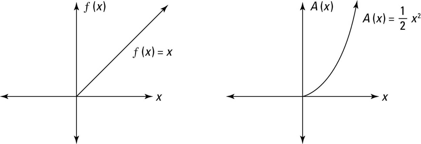
In comparison, look at Figure 3-8, which represents rising income. This time, I choose f(x) = x to represent income. This function produces the area function ![]() , which rises at an increasing rate.
, which rises at an increasing rate.
Figure 3-7: The function f(x) = 1 produces an area function A(x) = x.
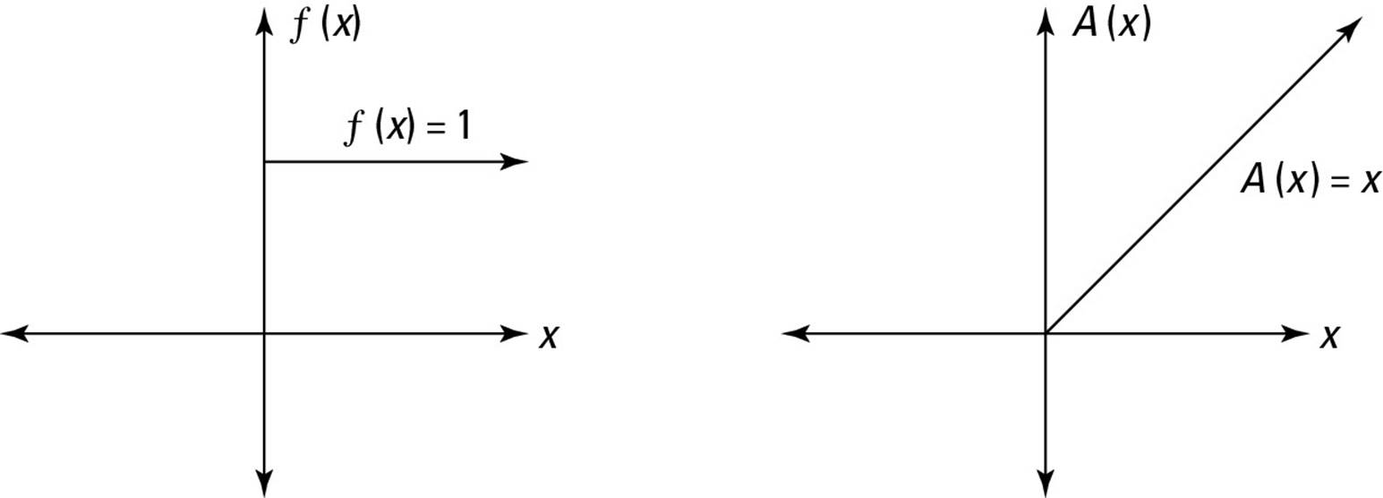
Figure 3-8: The function f(x) = xproduces an area function ![]() .
.
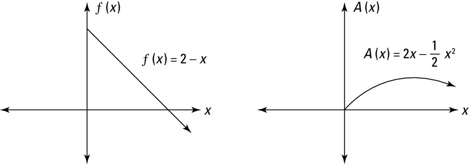
Finally, take a peek at Figure 3-9, which represents falling income. In this case, I use f(x) = 2 – x to represent income. This function results in the area function
![]() , which rises at a decreasing rate until the original function
, which rises at a decreasing rate until the original function
drops below 0, and then starts falling.
Take a moment to think about these three examples. Make sure that you see how, in a very practical sense, slope and area are connected: In other words, the slope of a function is the qualitative factor that governs what the related area function looks like.
Figure 3-9: The function f(x) = 2 – x produces an area function  .
.
Connecting slope and area mathematically
In the previous section, I discuss three functions f(x) and their related area functions A(x). Table 3-7 summarizes this information.
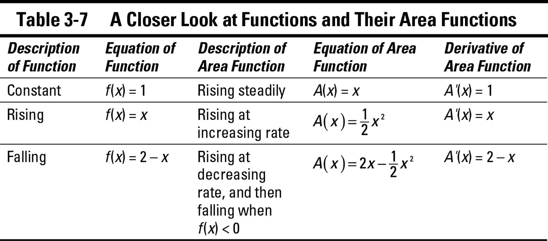
At this point, the big connection is only a heartbeat away. Notice that each function is the derivative of its area function:
A'(x) = f(x)
Is this mere coincidence? Not at all. Table 3-7 just adds mathematical precision to the intuitive idea that the slope of a function (that is, its derivative) is related to the area underneath it.
Because area is mathematically described by the definite integral, as I discuss in Chapter 1, this connection between differentiation and integration makes a whole lot of sense. That’s why finding the area under a function — that is, integration — is essentially undoing a derivative — that is, anti-differentiation.
Seeing a dark side of the FTC
Earlier in this chapter, I give you this piece of the Fundamental Theorem of Calculus:
![]()
Now that you understand the connection between a function f(x) and its area function A(x), here’s another piece of the FTC:
![]()
This piece of the theorem is generally regarded as less useful than the first piece, and it’s also harder to grasp because of all the extra variables. I won’t belabor it too much, but here are a few points that may help you understand it better:
![]() The variable s — the lower limit of integration — is an arbitrary starting point where the area function equals zero. In my examples in the previous section, I start the area function at the origin, so s = 0. This point represents the day when you opened your bank account, before you deposited any money.
The variable s — the lower limit of integration — is an arbitrary starting point where the area function equals zero. In my examples in the previous section, I start the area function at the origin, so s = 0. This point represents the day when you opened your bank account, before you deposited any money.
![]() The variable x — the upper limit of integration — represents any time after you opened your bank account. It’s also the independent variable of the area function.
The variable x — the upper limit of integration — represents any time after you opened your bank account. It’s also the independent variable of the area function.
![]() The variable t is the variable of the function. If you were to draw a graph, t would be the independent variable and f(t) the dependent variable.
The variable t is the variable of the function. If you were to draw a graph, t would be the independent variable and f(t) the dependent variable.
In short, don’t worry too much about this version of the FTC. The most important thing is that you remember the first version and know how to use it. The other important thing is that you understand how slope and area — that is, derivatives and integrals — are intimately related.
Your New Best Friend: The Indefinite Integral
The Fundamental Theorem of Calculus gives you insight into the connection between a function’s slope and the area underneath it — that is, between differentiation and integration.
On a practical level, the FTC gives you an easier way to integrate, without resorting to the Riemann sum formula. This easier way is called anti-differentiation — in other words, undoing differentiation. Anti-differentiation is the method that you’ll use to integrate throughout the remainder of Calculus II. It leads quickly to a new key concept: the indefinite integral.
In this section, I show you step by step how to use the indefinite integral to solve definite integrals, and I introduce the important concept of signed area. To finish the chapter, I make sure that you understand the important distinctions between definite and indefinite integrals.
Introducing anti-differentiation
Integration without resorting to the Riemann sum formula depends on undoing differentiation (anti-differentiation). Earlier in this chapter, in “Light at the End of the Tunnel: The Fundamental Theorem of Calculus,” I calculate a few areas informally by reversing a few differentiation formulas that you know from Calculus I. But anti-differentiation is so important that it deserves its own notation: the indefinite integral.
An indefinite integral is simply the notation representing the inverse of the derivative function:
![]()
 Be careful not to confuse the indefinite integral with the definite integral. For the moment, notice that the indefinite integral has no limits of integration. Later in this chapter, in “Distinguishing definite and indefinite integrals,” I outline the differences between these two types of integrals.
Here are a few examples that informally connect derivatives that you know with indefinite integrals that you want to be able to solve:
![]()
![]()
![]()
There’s a small but important catch in this informal analysis. Notice that the following three statements are all true:
![]()
![]()
![]()
Because any constant differentiates to 0, you need to account for the possible presence of a constant when integrating. So here are the more precise formulations of the indefinite integrals I just introduced:
![]()
![]()
![]()
 The formal solution of every indefinite integral is an anti-derivative up to the addition of a constant C, which is called the constant of integration. So just mechanically attach a + C whenever you evaluate an indefinite integral.
Solving area problems without the Riemann sum formula
After you know how to solve an indefinite integral by using anti-differentiation (as I show you in the previous section), you have at your disposal a useful method for solving area problems. This announcement should come as a great relief, especially after reading the earlier section “As Bad as It Gets: Calculating Definite Integrals Using the Riemann Sum Formula.”
Here’s how you solve an area problem using indefinite integrals — that is, without resorting to the Riemann sum formula:
1. Formulate the area problem as a definite integral (as I show you in Chapter 1).
2. Solve the definite integral as an indefinite integral evaluated between the given limits of integration.
3. Plug the limits of integration into this expression and simplify to find the area.
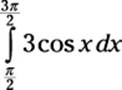
This method is, in fact, the one that you use for solving area problems for the rest of Calculus II. For example, suppose that you want to find the shaded area in Figure 3-10.
Figure 3-10:The shaded area  .
.
Here’s how you do it:
1. Formulate the area problem as a definite integral:
2. Solve this definite integral as an indefinite integral:
![]()
I replace the integral with the expression 3 sin x, because ![]() 3 sin x = 3 cos x. I also introduce the notation
3 sin x = 3 cos x. I also introduce the notation ![]() . You can read it as evaluated from x equals
. You can read it as evaluated from x equals ![]() to x equals
to x equals ![]() . This notation is commonly used so that you can show your teacher that you know how to integrate and postpone worrying about the limits of integration until the next step.
. This notation is commonly used so that you can show your teacher that you know how to integrate and postpone worrying about the limits of integration until the next step.
3. Plug these limits of integration into the expression and simplify:
![]()
As you can see, this step comes straight from the FTC, subtracting f(b) – f(a). Now I just simplify this expression to find the area:
= 3 – (–3) = 6
So the area of the shaded region in Figure 3-10 equals 6.
No C? No problem!
You may wonder why the constant of integration C — which is so important when you’re evaluating an indefinite integral — gets dropped when you’re evaluating a definite integral. This one is easy to explain.
Remember that every definite integral is expressed as the difference between a function evaluated at one point and the same function evaluated at another point. If this function includes a constant C, one C cancels out the other.
For example, take the definite integral ![]() . Technically speaking, this integral is evaluated as follows:
. Technically speaking, this integral is evaluated as follows:
![]()
![]()
![]()
As you can clearly see, the two Cs cancel each other out, so there’s no harm in dropping them at the beginning of the evaluation rather than at the end.
Understanding signed area
In the real world, the smallest possible area is 0, so area is always a nonnegative number. On the graph, however, area can be either positive or negative.
This idea of negative area relates back to a discussion earlier in this chapter, in “Introducing the area function,” where I talk about what happens when a function dips below the x-axis.
To use the analogy of income and savings, this is the moment when your income dries up and money starts flowing out. In other words, you’re spending your savings, so your savings account balance starts to fall. So area above the x-axis is positive, but area below the x-axis is measured as negative area.
The definite integral takes this important distinction into account. It provides not just the area but the signed area of a region on the graph. For example, suppose that you want to measure the shaded area in Figure 3-11.
Figure 3-11:Measuring signed area on the graph  .
.
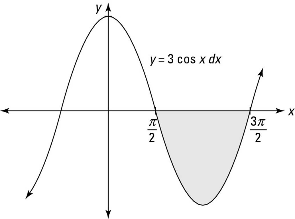
Here’s how you do it using the steps that I outline in the previous section:
1. Formulate the area problem as a definite integral:
2. Solve this definite integral as an indefinite integral:
![]()
3. Plug these limits of integration into the expression and simplify:
![]()
= –3 – 3 = –6
So the signed area of the shaded region in Figure 3-11 equals –6. As you can see, the computational method for evaluating the definite integral gives the signed area automatically.
As another example, suppose that you want to find the total area of the two shaded regions in Figure 3-10 and Figure 3-11. Here’s how you do it using the steps that I outline in the previous section:
1. Formulate the area problem as a definite integral:
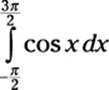
2. Solve this definite integral as an indefinite integral:
![]()
3. Plug these limits of integration into the expression and simplify:
![]()
= 3 – 3 = 0
This time, the signed area of the shaded region is 0. This answer makes sense, because the unsigned area above the x-axis equals the unsigned area below it, so these two areas cancel each other out.
Distinguishing definite and indefinite integrals
Don’t confuse the definite and indefinite integrals. Here are the key differences between them:
A definite integral
![]() Includes limits of integration (a and b)
Includes limits of integration (a and b)
![]() Represents the exact area of a specific set of points on a graph
Represents the exact area of a specific set of points on a graph
![]() Evaluates to a number
Evaluates to a number
An indefinite integral
![]() Doesn’t include limits of integration
Doesn’t include limits of integration
![]() Can be used to evaluate an infinite number of related definite integrals
Can be used to evaluate an infinite number of related definite integrals
![]() Evaluates to a function
Evaluates to a function
For example, here’s a definite integral:
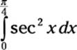
As you can see, it includes limits of integration (0 and ![]() ), so you can draw a graph of the area that it represents. You can then use a variety of methods to evaluate this integral as a number. This number equals the signed area between the function and the x-axis inside the limits of integration, as I discuss earlier in “Understanding signed area.”
), so you can draw a graph of the area that it represents. You can then use a variety of methods to evaluate this integral as a number. This number equals the signed area between the function and the x-axis inside the limits of integration, as I discuss earlier in “Understanding signed area.”
In contrast, here’s an indefinite integral:
![]()
This time, the integral doesn’t include limits of integration, so it doesn’t represent a specific area. Thus, it doesn’t evaluate to a number, but to a function:
= tan x + C
You can use this function to evaluate any related definite integral. For example, here’s how to use it to evaluate the definite integral I just gave you:
= ![]()
= ![]()
= 1 – 0 = 1
So the value of this definite integral is 1.
As you can see, the indefinite integral encapsulates an infinite number of related definite integrals. It also provides a practical means for evaluating definite integrals. Small wonder that much of Calculus II focuses on evaluating indefinite integrals. In Part II, I give you an ordered approach to evaluating indefinite integrals.