Calculus For Dummies, 2nd Edition (2014)
Part IV. Differentiation
Chapter 11. Differentiation and the Shape of Curves
IN THIS CHAPTER
Weathering the ups and downs of moody functions
Locating extrema
Using the first and second derivative tests
Interpreting concavity and points of inflection
Comparing the graphs of functions and derivatives
Muzzling the mean value theorem — GRRRRR
If you’ve read Chapters 9 and 10, you’re probably an expert at finding derivatives. Which is a good thing, because in this chapter you use derivatives to understand the shape of functions — where they rise and where they fall, where they max out and bottom out, how they curve, and so on. Then in Chapter 12, you use your knowledge about the shape of functions to solve real-world problems.
Taking a Calculus Road Trip
Consider the graph of ![]() in Figure 11-1.
in Figure 11-1.
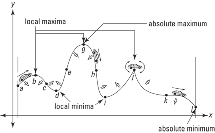
FIGURE 11-1: The graph of ![]() with several points of interest.
with several points of interest.
Imagine that you’re driving along this function from left to right. Along your drive, there are several points of interest between a and l. All of them, except for the start and finish points, relate to the steepness of the road — in other words, its slope or derivative.
Now, prepare yourself — I’m going to throw lots of new terms and definitions at you all at once here. You shouldn’t, however, have much trouble with these ideas because they mostly involve commonsense notions like driving up or down an incline, or going over the crest of a hill.
Climb every mountain, ford every stream: Positive and negative slopes
First, notice that as you begin your trip at a, you’re climbing up. Thus the function is increasing and its slope and derivative are therefore positive. You climb the hill till you reach the top at b where the road levels out. The road is level there, so the slope and derivative equal zero.
Because the derivative is zero at b, point b is called a stationary point of the function. Point b is also a local maximum or relative maximum of f because it’s the top of a hill. To be a local max, b just has to be the highest point in its immediate neighborhood. It doesn’t matter that the nearby hill at g is even higher.
After reaching the crest of the hill at b, you start going down — duh. So, after b, the slope and derivative are negative and the function is decreasing. To the left of every local max, the slope is positive; to the right of a max, the slope is negative.
I can’t think of a travel metaphor for this section: Concavity and inflection points
The next point of interest is c. Can you see that as you go down from b to c, the road gets steeper and steeper, but that after c, although you’re still going down, the road is gradually starting to curve up again and get less steep? The little down arrow between b and c in Figure 11-1 indicates that this section of the road is curving down — the function is said to be concave down there. As you can see, the road is also concave down between a and b.
 Concavity poetry: Down looks like a frown, up looks like a cup. A portion of a function that’s concave down looks like a frown. Where it’s concave up, like between c and e, it looks like a cup.
Wherever a function is concave down, its derivative (and slope) are decreasing; wherever a function is concave up, its derivative (and slope) are increasing.
Okay, so the road is concave down until c where it switches to concave up. Because the concavity switches at c, it’s a point of inflection. The point c is also the steepest point on this stretch of the road. Inflection points are always at the steepest — or least steep — points in their immediate neighborhoods.
 Be careful with function sections that have a negative slope. Point c is the steepest point in its neighborhood because it has a bigger negative slope than any other nearby point. But remember, a big negative number is actually a small number, so the slope and derivative at c are actually the smallest of all the points in the neighborhood. From b to c the derivative of the function is decreasing (because it’s becoming a bigger negative). From c to d, the derivative is increasing (because it’s becoming a smaller negative). Got it?
This vale of tears: A local minimum
Let’s get back to your drive. After point c, you keep going down till you reach d, the bottom of a valley. Point d is another stationary point because the road is level there and the derivative is zero. Point d is also a local or relative minimum because it’s the lowest point in its immediate neighborhood.
A scenic overlook: The absolute maximum
After d, you travel up, passing e, which is another inflection point. It’s the steepest point between d and g and the point where the derivative is greatest. You stop at the scenic overlook at g, another stationary point and another local max. Point g is also the absolute maximum on the interval from a to l because it’s the very highest point on the road from a to l.
Car trouble: Teetering on the corner
Going down from g, you pass another inflection point, h, another local min, i, then you go up to j where you foolishly try to drive over the peak. Your front wheels make it over, but your car’s chassis gets stuck on the precipice, leaving you teetering up and down with your wheels spinning. Your car teeters at j because you can’t draw a tangent line there. No tangent line means no slope; and no slope means no derivative, or you can say that the derivative at j is undefined. A sharp turning point like j is called a corner. (By the way, be careful with the expressions “no slope” and “no derivative.” In this context, “no” means nonexistent, NOT zero.)
It’s all downhill from here
After dislodging your car, you head down, the road getting less and less steep until it flattens out for an instant at k. (Again, note that because the slope and the derivative are becoming smaller and smaller negative numbers on the way to k, they are actually increasing.) Point k is another stationary point because its derivative is zero. It’s also another inflection point because the concavity switches from up to down at k. After passing k, you go down to l,your final destination. Because l is the endpoint of the interval, it’s not a local min — endpoints never qualify as local mins or maxes — but it is the absolute minimum on the interval because it’s the very lowest point from a to l.
Hope you enjoyed your trip.
Your travel diary
I want to review your trip and some of the previous terms and definitions and introduce yet a few more terms:
· The function f in Figure 11-1 has a derivative of zero at stationary points (level points) b, d, g, i, and k. At j, the derivative is undefined. These points where the derivative is either zero or undefined are the critical points of the function. The x-values of these critical points are called the critical numbers of the function. (Note that critical numbers must be within a function’s domain.)
· All local maxes and mins — the peaks and valleys — must occur at critical points. However, not all critical points are necessarily local maxes or mins. Point k, for instance, is a critical point but neither a max nor a min. Local maximums and minimums — or maxima and minima — are called, collectively, local extrema of the function. Use a lot of these fancy plurals if you want to sound like a professor. A single local max or min is a local extremum. The absolute max is the highest point on the road from a to l. The absolute min is the lowest point.
· The function is increasing whenever you’re going up, where the derivative is positive; it’s decreasing whenever you’re going down, where the derivative is negative. The function is also decreasing at point k, a horizontal inflection point, even though the slope and derivative are zero there. I realize that seems a bit odd, but that’s the way it works — take my word for it. At all horizontal inflection points, a function is either increasing or decreasing. At local extrema b, d, g, i, and j, the function is neither increasing nor decreasing.
· The function is concave up wherever it looks like a cup or a smile (some say where it “holds water”) and concave down wherever it looks like a frown (or “spills water”). Inflection points c, e, h, and k are where the concavity switches from up to down or vice versa. Inflection points are also the steepest or least steep points in their immediate neighborhoods.
Finding Local Extrema — My Ma, She’s Like, Totally Extreme
Now that you have the preceding section under your belt and know what local extrema are, you need to know how to do the math to find them. You saw in the last section that all local extrema occur at critical points of a function — that’s where the derivative is zero or undefined (but don’t forget that critical points aren’t always local extrema). So, the first step in finding a function’s local extrema is to find its critical numbers (the x-values of the critical points).
Cranking out the critical numbers
Find the critical numbers of ![]() . See Figure 11-2.
. See Figure 11-2.
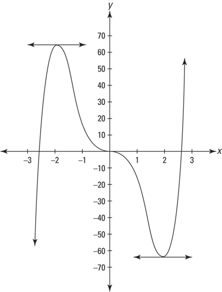
FIGURE 11-2: The graph of ![]() .
.
Here’s what you do:
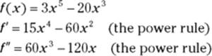
1. Find the first derivative of f using the power rule.
![]()
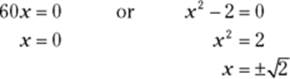
2. Set the derivative equal to zero and solve for x.
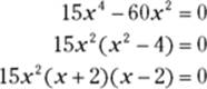
![]()
These three x-values are critical numbers of f. Additional critical numbers could exist if the first derivative were undefined at some x-values, but because the derivative, ![]() , is defined for all input values, the above solution set,
, is defined for all input values, the above solution set, ![]() is the complete list of critical numbers. Because the derivative of f equals zero at these three critical numbers, the curve has horizontal tangents at these numbers. In Figure 11-2, you can see the little horizontal tangent lines drawn where
is the complete list of critical numbers. Because the derivative of f equals zero at these three critical numbers, the curve has horizontal tangents at these numbers. In Figure 11-2, you can see the little horizontal tangent lines drawn where ![]() . The third horizontal tangent line where
. The third horizontal tangent line where ![]() is the x-axis.
is the x-axis.
 A curve has a horizontal tangent line wherever its derivative is zero, namely, at its stationary points. A curve will have horizontal tangent lines at all of its local mins and maxes (except for sharp corners like point j in Figure 11-1) and at all of its horizontal inflection points.
Now that you’ve got the list of critical numbers, you need to determine whether peaks or valleys or inflection points occur at those x-values. You can do this with either the first derivative test or the second derivative test. I suppose you may be wondering why you have to test the critical numbers when you can see where the peaks and valleys are by just looking at the graph in Figure 11-2 — which you can, of course, reproduce on your graphing calculator. Good point. Okay, so this problem — not to mention countless other problems you’ve done in math courses — is somewhat contrived and impractical. So what else is new?
The first derivative test
The first derivative test is based on the Nobel-Prize-caliber ideas that as you go over the top of a hill, first you go up and then you go down, and that when you drive into and out of a valley, you go down and then up. This calculus stuff is pretty amazing, isn’t it?
Here’s how you use the test. Take a number line and put down the critical numbers you found above: ![]() . See Figure 11-3.
. See Figure 11-3.
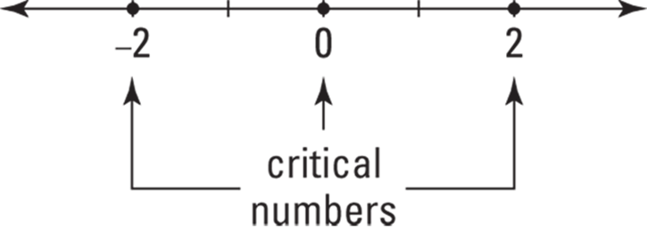
FIGURE 11-3: The critical numbers of ![]()
This number line is now divided into four regions: to the left of ![]() , from
, from ![]() to 0, from 0 to 2, and to the right of 2. Pick a value from each region, plug it into the first derivative, and note whether your result is positive or negative. Let’s use the numbers
to 0, from 0 to 2, and to the right of 2. Pick a value from each region, plug it into the first derivative, and note whether your result is positive or negative. Let’s use the numbers ![]() 1, and 3 to test the regions:
1, and 3 to test the regions:
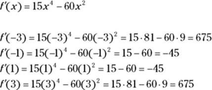
By the way, if you had noticed that this first derivative is an even function, you’d have known, without doing the computation, that ![]() and that
and that ![]() . (Chapter 5 discusses even functions. A polynomial function with all even powers, like
. (Chapter 5 discusses even functions. A polynomial function with all even powers, like ![]() above, is one type of even function.)
above, is one type of even function.)
These four results are, respectively, positive, negative, negative, and positive. Now, take your number line, mark each region with the appropriate positive or negative sign, and indicate where the function is increasing (where the derivative is positive) and decreasing (where the derivative is negative). The result is a so-called sign graph. See Figure 11-4. (The four right-pointing arrows at the top of the figure simply indicate that “increasing” and “decreasing” tell you what’s happening as you move along the function from left to right.)
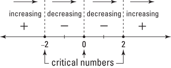
FIGURE 11-4: The sign graph for ![]()
Figure 11-4 simply tells you what you already know if you’ve looked at the graph of f — that the function goes up until ![]() , down from
, down from ![]() to 0, further down from 0 to 2, and up again from 2 on.
to 0, further down from 0 to 2, and up again from 2 on.
Now here’s the rocket science. The function switches from increasing to decreasing at ![]() ; in other words, you go up to
; in other words, you go up to ![]() and then down. So at
and then down. So at ![]() you have the top of a hill or a local maximum. Conversely, because the function switches from decreasing to increasing at 2, you have the bottom of a valley there or a local minimum. And because the sign of the first derivative doesn’t switch (from positive to negative or vice versa) at zero, there’s neither a min nor a max at that x-value (you usually — like here — get a horizontal inflection point when this happens).
you have the top of a hill or a local maximum. Conversely, because the function switches from decreasing to increasing at 2, you have the bottom of a valley there or a local minimum. And because the sign of the first derivative doesn’t switch (from positive to negative or vice versa) at zero, there’s neither a min nor a max at that x-value (you usually — like here — get a horizontal inflection point when this happens).
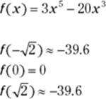
The last step is to obtain the function values, in other words the heights, of these two local extrema by plugging the x-values into the original function:
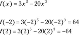
Thus, the local max is located at ![]() and the local min is at
and the local min is at ![]() . You’re done.
. You’re done.
Local extrema don’t occur at points of discontinuity. To use the first derivative test to test for a local extremum at a particular critical number, the function must be continuous at that x-value.
The second derivative test — no, no, anything but another test!
The second derivative test is based on two more prize-winning ideas: First, that at the crest of a hill, a road has a hump shape — in other words, it’s curving down or concave down; and second, that at the bottom of a valley, a road is cup-shaped, so it’s curving up or concave up.
The concavity of a function at a point is given by its second derivative: a positive second derivative means the function is concave up, a negative second derivative means the function is concave down, and a second derivative of zero is inconclusive (the function could be concave up, concave down, or there could be an inflection point there). So, for our function f, all you have to do is find its second derivative and then plug in the critical numbers you found, ![]() and note whether your results are positive, negative, or zero. To wit —
and note whether your results are positive, negative, or zero. To wit —
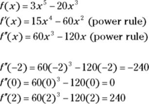
At ![]() , the second derivative is negative
, the second derivative is negative ![]() . This tells you that f is concave down where x equals
. This tells you that f is concave down where x equals ![]() , and therefore that there’s a local max there. The second derivative is positive (240) where x is 2, so f is concave up and thus there’s a local min at
, and therefore that there’s a local max there. The second derivative is positive (240) where x is 2, so f is concave up and thus there’s a local min at ![]() . Because the second derivative equals zero at
. Because the second derivative equals zero at ![]() , the second derivative test fails for that critical number — it tells you nothing about the concavity at
, the second derivative test fails for that critical number — it tells you nothing about the concavity at ![]() or whether there’s a local min or max there. When this happens, you have to use the first derivative test.
or whether there’s a local min or max there. When this happens, you have to use the first derivative test.
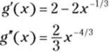
Now go through the first and second derivative tests one more time with another example. Find the local extrema of ![]() . See Figure 11-5.
. See Figure 11-5.
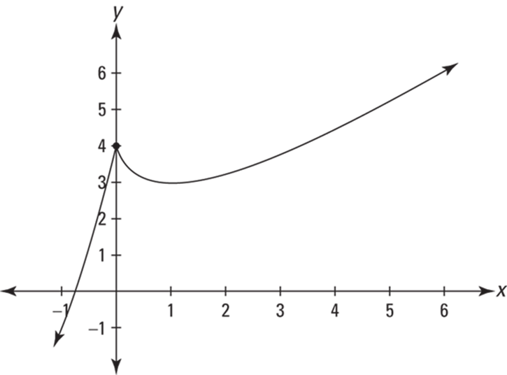
FIGURE 11-5: The graph of ![]()
![]()
1. Find the first derivative of g.
![]()
2. Set the derivative equal to zero and solve.
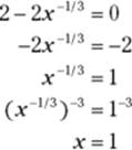
Thus 1 is a critical number.
3. Determine whether the first derivative is undefined for any x-values.
![]() equals
equals ![]() . Now, because the cube root of zero is zero, if you plug in zero to
. Now, because the cube root of zero is zero, if you plug in zero to ![]() , you’d have
, you’d have ![]() , which is undefined. So the derivative,
, which is undefined. So the derivative, ![]() , is undefined at
, is undefined at ![]() , and thus 0 is another critical number. From Steps 2 and 3, you’ve got the complete list of critical numbers of
, and thus 0 is another critical number. From Steps 2 and 3, you’ve got the complete list of critical numbers of ![]() and 1.
and 1.
4. Plot the critical numbers on a number line, and then use the first derivative test to figure out the sign of each region.
You can use ![]() as test numbers:
as test numbers:
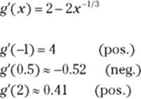
Figure 11-6 shows the sign graph.
Because the first derivative of g switches from positive to negative at 0, there’s a local max there. And because the first derivative switches from negative to positive at 1, there’s a local min at x = 1.
5. Plug the critical numbers into g to obtain the function values (the heights) of these two local extrema.
![]()
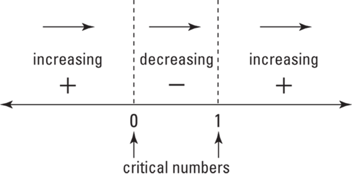
FIGURE 11-6: The sign graph of ![]()
![]()
So, there’s a local max at ![]() and a local min at
and a local min at ![]() . You’re done.
. You’re done.
You could have used the second derivative test instead of the first derivative test in Step 4. First, you need the second derivative of g, which is, as you know, the derivative of its first derivative:
Evaluate the second derivative at ![]() (the critical number from Step 2):
(the critical number from Step 2):
![]()
Because ![]() is positive, you know that g is concave up at
is positive, you know that g is concave up at ![]() and, therefore, that there’s a local min there.
and, therefore, that there’s a local min there.
At the other critical number, ![]() (from Step 3), the first derivative is undefined. The second derivative test is no help where the first derivative is undefined, so you’ve got to use the first derivative test for that critical number.
(from Step 3), the first derivative is undefined. The second derivative test is no help where the first derivative is undefined, so you’ve got to use the first derivative test for that critical number.
Finding Absolute Extrema on a Closed Interval
Every function that’s continuous on a closed interval has to have an absolute maximum value and an absolute minimum value in that interval — in other words, a highest and lowest point — though, as you see in the following example, there can be a tie for the highest or lowest value.
A closed interval like ![]() includes the endpoints 2 and 5. An open interval like
includes the endpoints 2 and 5. An open interval like ![]() excludes the endpoints.
excludes the endpoints.
Finding the absolute max and min is a snap. All you do is compute the critical numbers of the function in the given interval, determine the height of the function at each critical number, and then figure the height of the function at the two endpoints of the interval. The greatest of this set of heights is the absolute max; and the least, of course, is the absolute min. Here’s an example: Find the absolute max and min of ![]() in the closed interval
in the closed interval ![]() .
.
1. Find the critical numbers of h in the open interval ![]() .
.
(See Chapter 6 if you’re a little rusty on trig functions.)
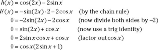
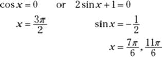
Thus, the zeros of ![]() are
are ![]() ,
, ![]() , and
, and ![]() , and because
, and because ![]() is defined for all input numbers, this is the complete list of critical numbers.
is defined for all input numbers, this is the complete list of critical numbers.
2. Compute the function values (the heights) at each critical number.
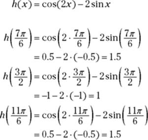
3. Determine the function values at the endpoints of the interval.
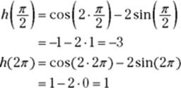
So, from Steps 2 and 3, you’ve found five heights: 1.5, 1, 1.5, ![]() , and 1. The largest number in this list, 1.5, is the absolute max; the smallest,
, and 1. The largest number in this list, 1.5, is the absolute max; the smallest, ![]() , is the absolute min.
, is the absolute min.
The absolute max occurs at two points: ![]() and
and ![]() . The absolute min occurs at one of the endpoints,
. The absolute min occurs at one of the endpoints, ![]() , and is thus called an endpoint extremum.
, and is thus called an endpoint extremum.
Table 11-1 shows the values of ![]() at the three critical numbers in the interval from
at the three critical numbers in the interval from ![]() to
to ![]() and at the interval’s endpoints; Figure 11-7 shows the graph of h.
and at the interval’s endpoints; Figure 11-7 shows the graph of h.
TABLE 11-1 Values of ![]() at the Critical Numbers and Endpoints for the Interval
at the Critical Numbers and Endpoints for the Interval ![]()
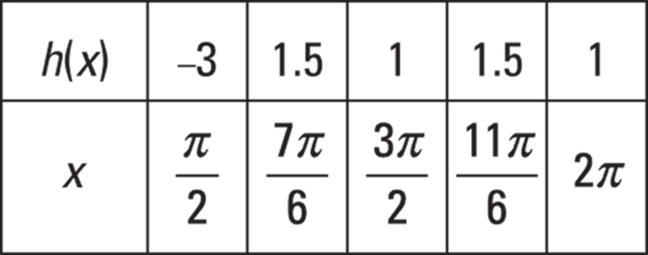
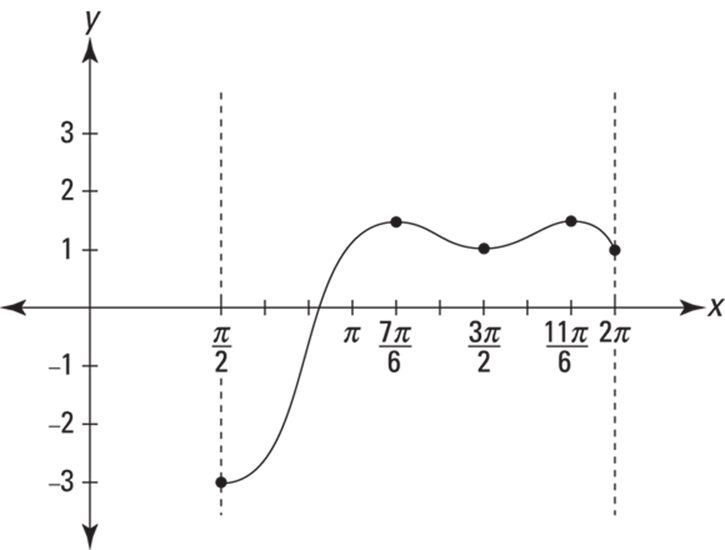
FIGURE 11-7: The graph of ![]()
A couple observations. First, as you can see in Figure 11-7, the points ![]() and
and ![]() are both local maxima of h, and the point
are both local maxima of h, and the point ![]() is a local minimum of h. However, if you want only to find the absoluteextrema on a closed interval, you don’t have to pay any attention to whether critical points are local maxes, mins, or neither. And thus you don’t have to bother to use the first or second derivative tests. All you have to do is determine the heights at the critical numbers and at the endpoints and then pick the largest and smallest numbers from this list. Second, the absolute max and min in the given interval tell you nothing about how the function behaves outside the interval. Function h, for instance, might rise higher than 1.5 outside the interval from
is a local minimum of h. However, if you want only to find the absoluteextrema on a closed interval, you don’t have to pay any attention to whether critical points are local maxes, mins, or neither. And thus you don’t have to bother to use the first or second derivative tests. All you have to do is determine the heights at the critical numbers and at the endpoints and then pick the largest and smallest numbers from this list. Second, the absolute max and min in the given interval tell you nothing about how the function behaves outside the interval. Function h, for instance, might rise higher than 1.5 outside the interval from ![]() to
to ![]() (although it doesn’t), and it might go lower than
(although it doesn’t), and it might go lower than ![]() (although it never does).
(although it never does).
Finding Absolute Extrema over a Function’s Entire Domain
A function’s absolute max and absolute min over its entire domain are the highest and lowest values (heights) of the function anywhere it’s defined. Unlike in the previous section where you saw that a continuous function must have both an absolute max and min on a closed interval, when you consider a function’s entire domain, a function can have an absolute max or min or both or neither. For example, the parabola ![]() has an absolute min at the point
has an absolute min at the point ![]() — the bottom of its cup shape — but no absolute max because it goes up forever to the left and the right. You might think that its absolute max would be infinity, but infinity is not a number and thus it doesn’t qualify as a maximum (ditto for using negative infinity as an absolute min).
— the bottom of its cup shape — but no absolute max because it goes up forever to the left and the right. You might think that its absolute max would be infinity, but infinity is not a number and thus it doesn’t qualify as a maximum (ditto for using negative infinity as an absolute min).
On the one hand, the idea of a function’s very highest point and very lowest point seems pretty simple, doesn’t it? But there’s a wrench in the works. The wrench is the category of things that don’t qualify as maxes or mins.
I already mentioned that infinity and negative infinity don’t qualify. Then there are empty “endpoints” like ![]() on
on ![]() in Figure 11-8.
in Figure 11-8. ![]() doesn’t have an absolute max. Its max isn’t 4 because it never gets to 4, and its max can’t be anything less than 4, like 3.999, because it gets higher than that, say 3.9999. Similarly, an infinitesimal hole in a function can’t qualify as a max or min. For example, consider the absolute value function,
doesn’t have an absolute max. Its max isn’t 4 because it never gets to 4, and its max can’t be anything less than 4, like 3.999, because it gets higher than that, say 3.9999. Similarly, an infinitesimal hole in a function can’t qualify as a max or min. For example, consider the absolute value function, ![]() , you know, the V-shaped function with the sharp corner at the origin; if you can’t picture it, look back at function g in Figure 7-8.
, you know, the V-shaped function with the sharp corner at the origin; if you can’t picture it, look back at function g in Figure 7-8. ![]() has no absolute max because it goes up to infinity. Its absolute min is zero (at
has no absolute max because it goes up to infinity. Its absolute min is zero (at ![]() of course). But now, say you alter the function slightly by plucking out the point at
of course). But now, say you alter the function slightly by plucking out the point at ![]() and leaving an infinitesimal hole there. Now the function has no absolute minimum.
and leaving an infinitesimal hole there. Now the function has no absolute minimum.
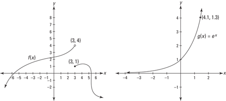
FIGURE 11-8: Two functions with no absolute extrema.
Now consider ![]() in Figure 11-8. It shows another type of situation that doesn’t qualify as a min (or max).
in Figure 11-8. It shows another type of situation that doesn’t qualify as a min (or max). ![]() has no absolute min. Going left, g crawls along the horizontal asymptote at
has no absolute min. Going left, g crawls along the horizontal asymptote at ![]() , always getting lower and lower, but never getting as low as zero. Since it never gets to zero, zero can’t be the absolute min, and there can’t be any other absolute min (like, say, 0.0001) because at some point way to the left, g will get below any small number you can name.
, always getting lower and lower, but never getting as low as zero. Since it never gets to zero, zero can’t be the absolute min, and there can’t be any other absolute min (like, say, 0.0001) because at some point way to the left, g will get below any small number you can name.
Keeping the above in mind, here’s a step-by-step approach for locating a function’s absolute maximum and minimum (if there are any):
1. Find the height of the function at each of its critical numbers. (Recall that a function’s critical numbers are the x-values within the function’s domain where the derivative is zero or undefined.)
You just did this in the previous section, but this time you consider all the critical numbers, not just those in a given interval. The highest of these values will be the function’s absolute max unless the function goes higher than that point in which case the function won’t have an absolute max. The lowest of those values will be the function’s absolute min unless the function goes lower than that point in which case it won’t have an absolute min. Steps 2 and 3 will help you figure out whether the function goes higher than the highest critical point and/or lower than the lowest critical point. If you apply Step 1 to ![]() in Figure 11-8, you’ll find that it has no critical points. When this happens, you’re done. The function has neither an absolute max nor an absolute min.
in Figure 11-8, you’ll find that it has no critical points. When this happens, you’re done. The function has neither an absolute max nor an absolute min.
2. Check whether the function goes up to infinity and/or down to negative infinity.
If a function goes up to positive infinity or down to negative infinity, it does so at its extreme right or left or at a vertical asymptote. So, evaluate ![]() and
and ![]() — the so-called end behavior of the function — and the limit of the function as x approaches each vertical asymptote (if there are any) from the left and from the right. If the function goes up to infinity, it has no absolute max; if it goes down to negative infinity, it has no absolute min.
— the so-called end behavior of the function — and the limit of the function as x approaches each vertical asymptote (if there are any) from the left and from the right. If the function goes up to infinity, it has no absolute max; if it goes down to negative infinity, it has no absolute min.
3. Graph the function to check for horizontal asymptotes and weird features like the jump discontinuity in ![]() in Figure 11-8.
in Figure 11-8.
Look at the graph of the function. If you see that the function gets higher than the highest of its critical points, it has no absolute max; if it goes lower than the lowest of its critical points, it has no absolute min. Applying this three-step process to ![]() in Figure 11-8, Step 1 would reveal two critical points: the endpoint at
in Figure 11-8, Step 1 would reveal two critical points: the endpoint at ![]() and the local max at roughly
and the local max at roughly ![]() . In Step 2, you would find that f goes down to negative infinity and thus has no absolute min. Finally, in Step 3, you’d see that f goes higher than the higher of the critical points,
. In Step 2, you would find that f goes down to negative infinity and thus has no absolute min. Finally, in Step 3, you’d see that f goes higher than the higher of the critical points, ![]() , and that it, therefore, has no absolute max. You’re done!
, and that it, therefore, has no absolute max. You’re done!
Locating Concavity and Inflection Points
Look back at the function ![]() in Figure 11-2. You used the three critical numbers of f,
in Figure 11-2. You used the three critical numbers of f, ![]() 0, and 2, to find the function’s local extrema:
0, and 2, to find the function’s local extrema: ![]() and
and ![]() . This section investigates what happens elsewhere on this function — specifically, where it’s concave up or down and where the concavity switches (the inflection points).
. This section investigates what happens elsewhere on this function — specifically, where it’s concave up or down and where the concavity switches (the inflection points).
The process for finding concavity and inflection points is analogous to using the first derivative test and the sign graph to find local extrema, except that now you use the second derivative. (See the section “Finding Local Extrema.”) Here’s what you do to find the intervals of concavity and the inflection points of ![]() :
:
1. Find the second derivative of f.
2. Set the second derivative equal to zero and solve.
![]()
3. Determine whether the second derivative is undefined for any x-values.
![]() is defined for all real numbers, so there are no other x-values to add to the list from Step 2. Thus, the complete list is
is defined for all real numbers, so there are no other x-values to add to the list from Step 2. Thus, the complete list is ![]() , 0, and
, 0, and ![]() .
.
Steps 2 and 3 give you what you could call “second derivative critical numbers” of f because they’re analogous to the critical numbers of f that you find using the first derivative. But, as far as I’m aware, this set of numbers has no special name. The important thing to know is that this list is made up of the zeros of ![]() plus any x-values where
plus any x-values where ![]() is undefined.
is undefined.
4. Plot these numbers on a number line and test the regions with the second derivative.
Use ![]() ,
, ![]() , 1, and 2 as test numbers.
, 1, and 2 as test numbers.
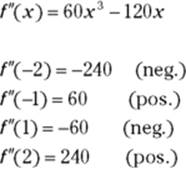
Figure 11-9 shows the sign graph.
A positive sign on this sign graph tells you that the function is concave up in that interval; negative means concave down. The function has an inflection point (usually) at any x-value where the signs switch from positive to negative or vice versa.
Because the signs switch at ![]() , 0, and
, 0, and ![]() , and because these three numbers are zeros of
, and because these three numbers are zeros of ![]() , inflection points occur at these x-values. If, however, you have a problem where the signs switch at a number where
, inflection points occur at these x-values. If, however, you have a problem where the signs switch at a number where ![]() is undefined, you have to check one additional thing before concluding that there’s an inflection point there. An inflection point exists at a given x-value only if you can draw a tangent line to the function at that number. This is the case if the first derivative exists at that number or if the tangent line is vertical there.
is undefined, you have to check one additional thing before concluding that there’s an inflection point there. An inflection point exists at a given x-value only if you can draw a tangent line to the function at that number. This is the case if the first derivative exists at that number or if the tangent line is vertical there.
5. Plug these three x-values into f to obtain the function values of the three inflection points.
The square root of two equals about 1.4, so there are inflection points at about ![]() ,
, ![]() , and about
, and about ![]() . You’re done.
. You’re done.
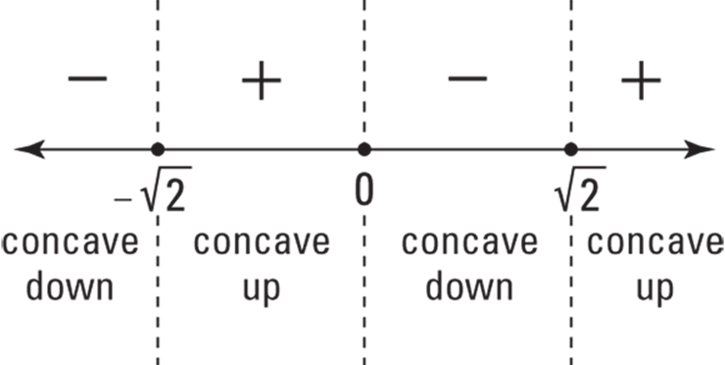
FIGURE 11-9: A second derivative sign graph for ![]()
Figure 11-10 shows f’s inflection points as well as its local extrema and its intervals of concavity.
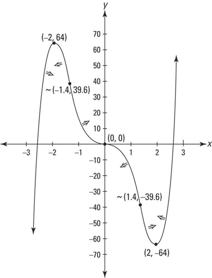
FIGURE 11-10: A graph of ![]() showing its local extrema, its inflection points, and its intervals of concavity.
showing its local extrema, its inflection points, and its intervals of concavity.
Looking at Graphs of Derivatives Till They Derive You Crazy
You can learn a lot about functions and their derivatives by looking at their graphs side by side and comparing their important features. Let’s keep going with the same function, ![]() ; we’re going to travel along ffrom left to right (see Figure 11-11), pausing to note its points of interest and also observing what’s happening to the graph of
; we’re going to travel along ffrom left to right (see Figure 11-11), pausing to note its points of interest and also observing what’s happening to the graph of ![]() at the same points. But first, check out the (long) warning beneath the figure.
at the same points. But first, check out the (long) warning beneath the figure.
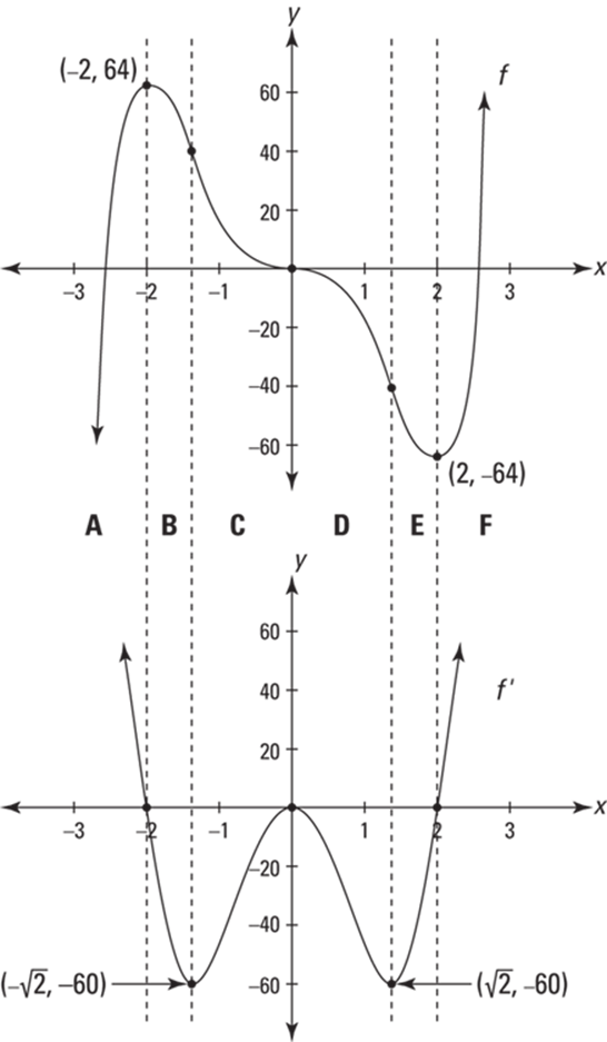
FIGURE 11-11: ![]() and its first derivative,
and its first derivative, ![]()
This is NOT the function! As you look at the graph of ![]() in Figure 11-11, or the graph of any other derivative, you may need to slap yourself in the face every minute or so to remind yourself that “This is the derivativeI’m looking at, not the function” You’ve looked at hundreds and hundreds of graphs of functions over the years, so when you start looking at graphs of derivatives, you can easily lapse into thinking of them as regular functions. You might, for instance, look at an interval that’s going up on the graph of a derivative and mistakenly conclude that the original function must also be going up in the same interval — an understandable mistake. You know the first derivative is the same thing as slope. So when you see the graph of the first derivative going up, you may think, “Oh, the first derivative (the slope) is going up, and when the slope goes up that’s like going up a hill, so the original function must be rising.” This sounds reasonable because, loosely speaking, you can describe the front side of a hill as a slope that’s going up, increasing. But mathematically speaking, the front side of a hill has a positive slope, not necessarily an increasing slope. So, where a function is increasing, the graph of its derivative will be positive, but that derivative graph might be going up or down. Say you’re going up a hill. As you approach the top of the hill, you’re still going up, but, in general, the slope (the steepness) is going down. It might be 3, then 2, then 1, and then, at the top of the hill, the slope is zero. So the slope is getting smaller or decreasing, even as you’re climbing the hill or increasing. In such an interval, the graph of the function is increasing, but the graph of its derivative is decreasing. Got that?
in Figure 11-11, or the graph of any other derivative, you may need to slap yourself in the face every minute or so to remind yourself that “This is the derivativeI’m looking at, not the function” You’ve looked at hundreds and hundreds of graphs of functions over the years, so when you start looking at graphs of derivatives, you can easily lapse into thinking of them as regular functions. You might, for instance, look at an interval that’s going up on the graph of a derivative and mistakenly conclude that the original function must also be going up in the same interval — an understandable mistake. You know the first derivative is the same thing as slope. So when you see the graph of the first derivative going up, you may think, “Oh, the first derivative (the slope) is going up, and when the slope goes up that’s like going up a hill, so the original function must be rising.” This sounds reasonable because, loosely speaking, you can describe the front side of a hill as a slope that’s going up, increasing. But mathematically speaking, the front side of a hill has a positive slope, not necessarily an increasing slope. So, where a function is increasing, the graph of its derivative will be positive, but that derivative graph might be going up or down. Say you’re going up a hill. As you approach the top of the hill, you’re still going up, but, in general, the slope (the steepness) is going down. It might be 3, then 2, then 1, and then, at the top of the hill, the slope is zero. So the slope is getting smaller or decreasing, even as you’re climbing the hill or increasing. In such an interval, the graph of the function is increasing, but the graph of its derivative is decreasing. Got that?
Okay, let’s get back to the f and its derivative in Figure 11-11. Beginning on the left and traveling toward the right, f increases until the local max at ![]() . It’s going up, so its slope is positive, but f is getting less and less steep so its slope is decreasing — the slope decreases until it becomes zero at the peak. This corresponds to the graph of
. It’s going up, so its slope is positive, but f is getting less and less steep so its slope is decreasing — the slope decreases until it becomes zero at the peak. This corresponds to the graph of ![]() (the slope) which is positive (because it’s above the x-axis) but decreasing as it goes down to the point
(the slope) which is positive (because it’s above the x-axis) but decreasing as it goes down to the point ![]() . Let’s summarize your entire trip along f and
. Let’s summarize your entire trip along f and ![]() with the following list of rules.
with the following list of rules.
Rules are rules:
· An increasing interval on a function corresponds to an interval on the graph of its derivative that’s positive (or zero for a single point if the function has a horizontal inflection point). In other words, a function’s increasing interval corresponds to a part of the derivative graph that’s above the x-axis (or that touches the axis for a single point in the case of a horizontal inflection point). See intervals A and F in Figure 11-11.
· A local max on the graph of a function (like ![]() corresponds to a zero (an x-intercept) on an interval of the graph of its derivative that crosses the x-axis going down (like at
corresponds to a zero (an x-intercept) on an interval of the graph of its derivative that crosses the x-axis going down (like at ![]() ).
).
 On a derivative graph, you’ve got an m-axis. When you’re looking at various points on the derivative graph, don’t forget that the y-coordinate of a point, like
 ![]() , on a graph of a first derivative tells you the slope of the original function, not its height. Think of the y-axis on the first derivative graph as the slope-axis or the m-axis; you could think of general points on the first derivative graph as having coordinates
, on a graph of a first derivative tells you the slope of the original function, not its height. Think of the y-axis on the first derivative graph as the slope-axis or the m-axis; you could think of general points on the first derivative graph as having coordinates ![]() .
.
· A decreasing interval on a function corresponds to a negative interval on the graph of the derivative (or zero for a single point if the function has a horizontal inflection point). The negative interval on the derivative graph is below the x-axis (or in the case of a horizontal inflection point, the derivative graph touches the x-axis at a single point). See intervals B, C, D, and E in Figure 11-11 (but consider them as a single section), where f goes down all the way from the local max at ![]() to the local min at
to the local min at ![]() and where
and where ![]() is negative between
is negative between ![]() and
and ![]() except for at the point
except for at the point ![]() on
on ![]() which corresponds to the horizontal inflection point on f.
which corresponds to the horizontal inflection point on f.
· A local min on the graph of a function corresponds to a zero (an x-intercept) on an interval of the graph of its derivative that crosses the x-axis going up (like at ![]() ).
).
Now let’s take a second trip along f to consider its intervals of concavity and its inflection points. First, consider intervals A and B in Figure 11-11. The graph of f is concave down — which means the same thing as a decreasingslope — until it gets to the inflection point at about ![]() .
.
So, the graph of ![]() decreases until it bottoms out at about
decreases until it bottoms out at about ![]() . These coordinates tell you that the inflection point at
. These coordinates tell you that the inflection point at ![]() on f has a slope of
on f has a slope of ![]() Note that the inflection point on f at
Note that the inflection point on f at ![]() is the steepest point on that stretch of the function, but it has the smallest slope because its slope is a larger negative than the slope at any other nearby point.
is the steepest point on that stretch of the function, but it has the smallest slope because its slope is a larger negative than the slope at any other nearby point.
Between ![]() and the next inflection point at
and the next inflection point at ![]() , f is concave up, which means the same thing as an increasing slope. So the graph of
, f is concave up, which means the same thing as an increasing slope. So the graph of ![]() increases from about
increases from about ![]() to where it hits a local max at
to where it hits a local max at ![]() . See interval C in Figure 11-11. Let’s take a break from our trip for some more rules.
. See interval C in Figure 11-11. Let’s take a break from our trip for some more rules.
More rules:
· A concave down interval on the graph of a function corresponds to a decreasing interval on the graph of its derivative (intervals A, B, and D in Figure 11-11). And a concave up interval on the function corresponds to an increasing interval on the derivative (intervals C, E, and F).
· An inflection point on a function (except for a vertical inflection point where the derivative is undefined) corresponds to a local extremum on the graph of its derivative. An inflection point of minimum slope (in its neighborhood) corresponds to a local min on the derivative graph; an inflection point of maximum slope (in its neighborhood) corresponds to a local max on the derivative graph.
Resuming our trip, after ![]() , f is concave down till the inflection point at about
, f is concave down till the inflection point at about ![]() — this corresponds to the decreasing section of
— this corresponds to the decreasing section of ![]() from
from ![]() to its min at
to its min at ![]() (interval D in Figure 11-11). Finally, f is concave up the rest of the way, which corresponds to the increasing section of
(interval D in Figure 11-11). Finally, f is concave up the rest of the way, which corresponds to the increasing section of ![]() beginning at
beginning at ![]() (intervals E and F in the figure).
(intervals E and F in the figure).
Well, that pretty much brings you to the end of the road. Going back and forth between the graphs of a function and its derivative can be very trying at first. If your head starts to spin, take a break and come back to this stuff later.
If I haven’t already succeeded in deriving you crazy — aren’t these calculus puns fantastic? — perhaps this final point will do the trick. Look again at the graph of the derivative, ![]() , in Figure 11-11 and also at the sign graph for
, in Figure 11-11 and also at the sign graph for ![]() in Figure 11-9. That sign graph, because it’s a second derivative sign graph, bears exactly (well, almost exactly) the same relationship to the graph of
in Figure 11-9. That sign graph, because it’s a second derivative sign graph, bears exactly (well, almost exactly) the same relationship to the graph of ![]() as a first derivative sign graph bears to the graph of a regular function. In other words, negative intervals on the sign graph in Figure 11-9 (to the left of
as a first derivative sign graph bears to the graph of a regular function. In other words, negative intervals on the sign graph in Figure 11-9 (to the left of ![]() and between 0 and
and between 0 and ![]() ) show you where the graph of
) show you where the graph of ![]() is decreasing; positive intervals on the sign graph (between
is decreasing; positive intervals on the sign graph (between ![]() and 0 and to the right of
and 0 and to the right of ![]() ) show you where
) show you where ![]() is increasing. And points where the signs switch from positive to negative or vice versa (at
is increasing. And points where the signs switch from positive to negative or vice versa (at ![]() , 0, and
, 0, and ![]() ) show you where
) show you where ![]() has local extrema. Clear as mud, right?
has local extrema. Clear as mud, right?
The Mean Value Theorem — GRRRRR
You won’t use the mean value theorem a lot, but it’s a famous theorem — one of the two or three most important in all of calculus — so you really should learn it. It’s very simple and has a nice connection to the mean value theorem for integrals which I show you in Chapter 17. Look at Figure 11-12.
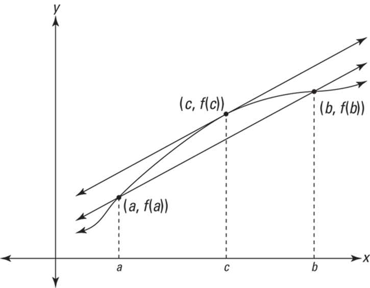
FIGURE 11-12: An Illustration of the mean value theorem.
Here’s the formal definition of the theorem.
The mean value theorem: If f is continuous on the closed interval ![]() and differentiable on the open interval
and differentiable on the open interval ![]() then there exists at least one number c in
then there exists at least one number c in ![]() such that
such that
![]()
Now for the plain-English version. First you need to take care of the fine print. The requirements in the theorem that the function be continuous and differentiable just guarantee that the function is a regular, smooth function without gaps or corners. But because only a few weird functions have gaps or corners, you don’t often have to worry about these fine points.
Here’s what the theorem means. The secant line connecting points ![]() and
and ![]() in Figure 11-12 has a slope given by the slope formula:
in Figure 11-12 has a slope given by the slope formula:
Note that this is the same as the right side of the equation in the mean value theorem. The derivative at a point is the same thing as the slope of the tangent line at that point, so the theorem just says that there must be at least one point between a and b where the slope of the tangent is the same as the slope of the secant line from a to b. The result is parallel lines, like in Figure 11-12.
Why must this be so? Here’s a visual argument. Imagine that you grab the secant line connecting ![]() and
and ![]() , and then you slide it up, keeping it parallel to the original secant line. Can you see that the two points of intersection between this sliding line and the function — the two points that begin at
, and then you slide it up, keeping it parallel to the original secant line. Can you see that the two points of intersection between this sliding line and the function — the two points that begin at ![]() and
and ![]() — will gradually get closer and closer to each other until they come together at
— will gradually get closer and closer to each other until they come together at ![]() ? If you raise the line any further, you break away from the function entirely. At this last point of intersection,
? If you raise the line any further, you break away from the function entirely. At this last point of intersection, ![]() , the sliding line touches the function at a single point and is thus tangent to the function there, and it has the same slope as the original secant line. Well, that does it. This explanation is a bit oversimplified, but it’ll do.
, the sliding line touches the function at a single point and is thus tangent to the function there, and it has the same slope as the original secant line. Well, that does it. This explanation is a bit oversimplified, but it’ll do.
Here’s a completely different sort of argument that should appeal to your common sense. If the function in Figure 11-12 gives your car’s odometer reading as a function of time, then the slope of the secant line from a to b gives your average speed during that interval of time, because dividing the distance traveled, ![]() , by the elapsed time,
, by the elapsed time, ![]() , gives you the average speed. The point
, gives you the average speed. The point ![]() , guaranteed by the mean value theorem, is a point where your instantaneous speed — given by the derivative
, guaranteed by the mean value theorem, is a point where your instantaneous speed — given by the derivative ![]() — equals your average speed.
— equals your average speed.
Now, imagine that you take a drive and average 50 miles per hour. The mean value theorem guarantees that you are going exactly 50 mph for at least one moment during your drive. Think about it. Your average speed can’t be 50 mph if you go slower than 50 the whole way or if you go faster than 50 the whole way. To average 50 mph, either you go exactly 50 for the whole drive, or you have to go slower than 50 for part of the drive and faster than 50 at other times. And if you’re going less than 50 at one point and more than 50 at a later point (or vice versa), you’ve got to hit exactly 50 at least once as you speed up (or slow down). You can’t jump over 50 — like going 49 one moment then 51 the next — because speeds go up by sliding up the scale, not jumping. At some point your speedometer slides past 50, and for at least one instant, you’re going exactly 50 mph. That’s all the mean value theorem says.