Calculus For Dummies, 2nd Edition (2014)
Part IV. Differentiation
Chapter 13. More Differentiation Problems: Going Off on a Tangent
IN THIS CHAPTER
Tangling with tangents
Negotiating normals
Lining up for linear approximations
Profiting from business and economics problems
In this chapter, you see three more applications of differentiation: tangent and normal line problems, linear approximation problems, and economics problems. The common thread tying these problems together is the idea of a line tangent to a curve — which should come as no surprise since the meaning of the derivative of a curve is the slope of the tangent line.
Tangents and Normals: Joined at the Hip
By now you know what a line tangent to a curve looks like — if not, one or both of us has definitely dropped the ball. A normal line is simply a line perpendicular to a tangent line at the point of tangency. Problems involving tangents and normals are common applications of differentiation.
The tangent line problem
I bet there have been several times, just in the last month, when you’ve wanted to determine the location of a line through a given point that’s tangent to a given curve. Here’s how you do it.
Example: Determine the points of tangency of the lines through the point ![]() that are tangent to the parabola
that are tangent to the parabola ![]() .
.
Solution: If you graph the parabola and plot the point, you can see that there are two ways to draw a tangent line from ![]() : up to the right and up to the left. See Figure 13-1.
: up to the right and up to the left. See Figure 13-1.
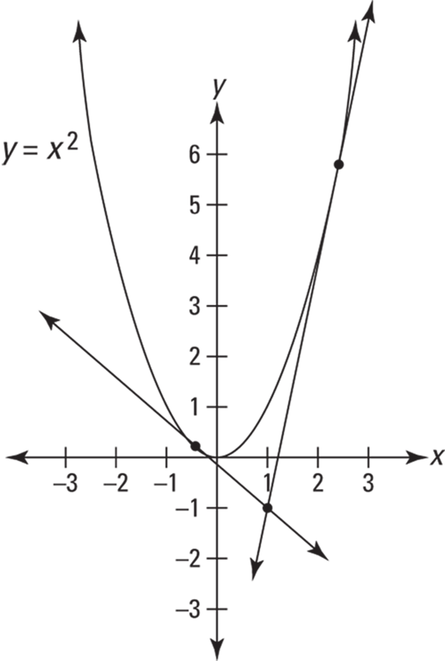
FIGURE 13-1: The parabola ![]() and two tangent lines through
and two tangent lines through ![]() .
.
The key to this problem is in the meaning of the derivative: Don’t forget — The derivative of a function at a given point is the slope of the tangent line at that point. So, all you have to do is set the derivative of the parabola equal to the slope of the tangent line and solve:
1. Because the equation of the parabola is ![]() , you can take a general point on the parabola,
, you can take a general point on the parabola, ![]() , and substitute
, and substitute ![]() for y.
for y.
So, label the two points of tangency ![]() .
.
2. Take the derivative of the parabola.
![]()
3. Using the slope formula, ![]() , set the slope of each tangent line from
, set the slope of each tangent line from ![]() to
to ![]() equal to the derivative at
equal to the derivative at ![]() which is 2x, and solve for x.
which is 2x, and solve for x.
(By the way, the math you do in this step may make more sense to you if you think of it as applying to just one of the tangent lines — say the one going up to the right — but the math actually applies to both tangent lines simultaneously.)
![]()
So, the x-coordinates of the points of tangency are ![]() and
and ![]() .
.
4. Plug each of these x-coordinates into ![]() to obtain the y-coordinates.
to obtain the y-coordinates.
|
|
|
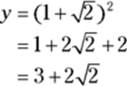
5. Thus, the two points of tangency are ![]() and
and ![]() , or about
, or about ![]() and
and ![]() .
.
The normal line problem
Here’s the companion problem to the tangent line problem in the previous section. Find the points of perpendicularity for all normal lines to the parabola, ![]() , that pass through the point
, that pass through the point ![]() .
.
 Definition of normal line: A line normal to a curve at a given point is the line perpendicular to the line that’s tangent to the curve at that same point.
Graph the parabola and plot the point ![]() . Now, before you do the math, try to estimate the locations of all normal lines. How many can you see? It’s fairly easy to see that, starting at
. Now, before you do the math, try to estimate the locations of all normal lines. How many can you see? It’s fairly easy to see that, starting at ![]() , one normal line goes down and to the right and another goes down to the left. But did you see that there’s actually a second normal line that goes down to the left? No worries if you didn’t see it, because when you do the math, you get all three solutions.
, one normal line goes down and to the right and another goes down to the left. But did you see that there’s actually a second normal line that goes down to the left? No worries if you didn’t see it, because when you do the math, you get all three solutions.
 Making commonsense estimates enhances mathematical understanding. When doing calculus, or any math for that matter, come up with a common sense, ballpark estimate of the solution to a problem before doing the math (when possible and time permitting). This deepens your understanding of the concepts involved and provides a check to the mathematical solution. (This is a powerful math strategy — take my word for it — despite the fact that in this particular problem, most people will find at most two of the three normal lines using an eyeball estimate.)
Figure 13-2 shows the parabola and the three normal lines.
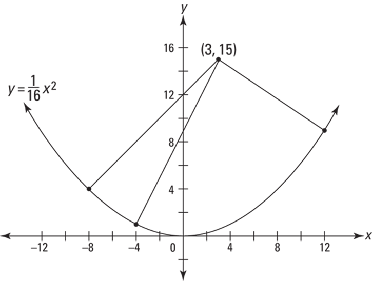
FIGURE 13-2: The parabola ![]() and three normal lines through
and three normal lines through ![]() .
.
Looking at the figure, you can appreciate how practical this problem is. It’ll really come in handy if you happen to find yourself standing inside the curve of a parabolic wall, and you want to know the precise location of the three points on the wall where you could throw a ball and have it bounce straight back to you.
The solution is very similar to the solution of the tangent line problem, except that in this problem you use the rule for perpendicular lines:
Slopes of perpendicular lines. The slopes of perpendicular lines are opposite reciprocals.
Each normal line in Figure 13-2 is perpendicular to the tangent line drawn at the point where the normal meets the curve. So the slope of each normal line is the opposite reciprocal of the slope of the corresponding tangent line — which, of course, is given by the derivative. So here goes:
1. Take a general point, ![]() , on the parabola
, on the parabola ![]() , and substitute
, and substitute ![]() for y.
for y.
So, label each point of perpendicularity ![]() .
.
2. Take the derivative of the parabola.

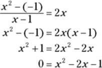
3. Using the slope formula, ![]() , set the slope of each normal line from
, set the slope of each normal line from ![]() to
to ![]() equal to the opposite reciprocal of the derivative at
equal to the opposite reciprocal of the derivative at ![]() , and solve for x.
, and solve for x.
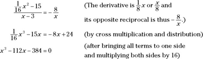
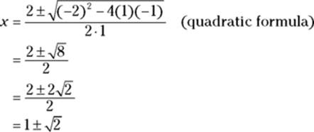
Now, there’s no easy way to get exact solutions to this cubic (3rd degree) equation like the way the quadratic formula gives you the exact solutions to a 2nd degree equation. Instead, you can graph ![]() , and the x-intercepts give you the solutions, but with this method, there’s no guarantee you’ll get exact solutions. (If you don’t, the decimal approximations you get will be good enough.) Here, however, you luck out — actually, I had something to do with it — and get the exact solutions of
, and the x-intercepts give you the solutions, but with this method, there’s no guarantee you’ll get exact solutions. (If you don’t, the decimal approximations you get will be good enough.) Here, however, you luck out — actually, I had something to do with it — and get the exact solutions of ![]()
![]() and 12. (You should graph the cubic function so you see how this works.)
and 12. (You should graph the cubic function so you see how this works.)
4. Plug each of these x-coordinates into ![]() to obtain the y-coordinates.
to obtain the y-coordinates.
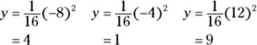
Thus, the three points of normalcy are ![]() ,
, ![]() , and
, and ![]() — play ball!
— play ball!
Straight Shooting with Linear Approximations
Because ordinary functions are locally linear (that’s straight) — and the further you zoom in on them, the straighter they look — a line tangent to a function is a good approximation of the function near the point of tangency. Figure 13-3 shows the graph of ![]() and a line tangent to the function at the point
and a line tangent to the function at the point ![]() . You can see that near
. You can see that near ![]() , the curve and the tangent line are virtually indistinguishable.
, the curve and the tangent line are virtually indistinguishable.
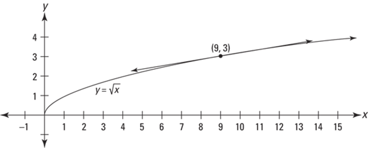
FIGURE 13-3: The graph of ![]() and a line tangent to the curve at
and a line tangent to the curve at ![]()
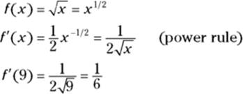
Determining the equation of this tangent line is a breeze. You’ve got a point, ![]() , and the slope is given by the derivative of f at 9:
, and the slope is given by the derivative of f at 9:
Now just take this slope (this derivative) of ![]() and the point
and the point ![]() , and plug them into point-slope form:
, and plug them into point-slope form:
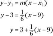
That’s the equation of the line tangent to ![]() at
at ![]() . I suppose you may be wondering why I wrote the equation as
. I suppose you may be wondering why I wrote the equation as ![]() . It might seem more natural to put the 3 to the right of
. It might seem more natural to put the 3 to the right of ![]() , which, of course, would also be correct. And I could have simplified the equation further, writing it in
, which, of course, would also be correct. And I could have simplified the equation further, writing it in ![]() form. I explain later in this section why I wrote it the way I did.
form. I explain later in this section why I wrote it the way I did.
(If you have your graphing calculator handy, graph ![]() and the tangent line. Zoom in on the point
and the tangent line. Zoom in on the point ![]() a couple times. You’ll see that — as you zoom in — the curve gets straighter and straighter and the curve and tangent line get closer and closer to each other.)
a couple times. You’ll see that — as you zoom in — the curve gets straighter and straighter and the curve and tangent line get closer and closer to each other.)
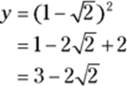
Now, say you want to approximate the square root of 10. Because 10 is pretty close to 9, and because you can see from Figure 13-3 that ![]() and its tangent line are close to each other at
and its tangent line are close to each other at ![]() , the y-coordinate of the line at
, the y-coordinate of the line at ![]() is a good approximation of the function value at
is a good approximation of the function value at ![]() , namely
, namely ![]() .
.
Just plug 10 into the line equation for your approximation:
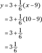
Thus, the square root of 10 is about ![]() . This is only about 0.004 more than the exact answer of 3.1623… . The error is roughly a tenth of a percent.
. This is only about 0.004 more than the exact answer of 3.1623… . The error is roughly a tenth of a percent.
Now I can explain why I wrote the equation for the tangent line the way I did. This form makes it easier to do the computation and easier to understand what’s going on when you compute an approximation. Here’s why. You know that the line goes through the point ![]() . right? And you know the slope of the line is
. right? And you know the slope of the line is ![]() . So, you can start at
. So, you can start at ![]() and go to the right (or left) along the line in the stair-step fashion, as shown in Figure 13-4: over 1, up
and go to the right (or left) along the line in the stair-step fashion, as shown in Figure 13-4: over 1, up ![]() ; over 1, up
; over 1, up ![]() ; and so on. (Note that since
; and so on. (Note that since ![]() , when the run is 1 (as shown in Figure 13-4), the rise equals the slope.)
, when the run is 1 (as shown in Figure 13-4), the rise equals the slope.)
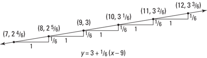
FIGURE 13-4: The linear approximation line and several of its points.
So, when you’re doing an approximation, you start at a y-value of 3 and go up ![]() for each 1 you go to the right. Or if you go to the left, you go down
for each 1 you go to the right. Or if you go to the left, you go down ![]() for each 1 you go to the left. When the line equation is written in the above form, the computation of an approximation parallels this stair-step scheme.
for each 1 you go to the left. When the line equation is written in the above form, the computation of an approximation parallels this stair-step scheme.
Figure 13-4 shows the approximate values for the square roots of 7, 8, 10, 11, and 12. Here’s how you come up with these values. To get to 8, for example, from ![]() , you go 1 to the left, so you go down
, you go 1 to the left, so you go down ![]() to
to ![]() ; or to get to 11 from
; or to get to 11 from ![]() , you go two to the right, so you go up two-sixths to
, you go two to the right, so you go up two-sixths to ![]() . (If you go to the right one half to
. (If you go to the right one half to ![]() , you go up half of a sixth, that’s a twelfth, to
, you go up half of a sixth, that’s a twelfth, to ![]() , the approximate square root of
, the approximate square root of ![]() .)
.)
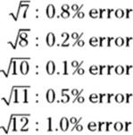
The following list shows the size of the errors for the approximations shown in Figure 13-4. Note that the errors grow as you get further from the point of tangency ![]() . Also, the errors grow faster going down from 9 to 8 then 7, etc. than going up from 9 to 10 then 11, etc.; errors often grow faster in one direction than the other with linear approximations because of the shape of the curve.
. Also, the errors grow faster going down from 9 to 8 then 7, etc. than going up from 9 to 10 then 11, etc.; errors often grow faster in one direction than the other with linear approximations because of the shape of the curve.
 Linear approximation equation: Here’s the general form for the equation of the tangent line that you use for a linear approximation. The values of a function
 ![]() can be approximated by the values of the tangent line
can be approximated by the values of the tangent line ![]() near the point of tangency,
near the point of tangency, ![]() , where
, where
![]()
This is less complicated than it looks. It’s just the gussied-up calculus version of the point-slope equation of a line you’ve known since Algebra I, ![]() , with the
, with the ![]() moved to the right side:
moved to the right side:
![]()
This equation and the equation for ![]() differ only in the symbols used; the meaning of both equations — term for term — is identical. And notice how they both resemble the equation of the tangent line in Figure 13-4.
differ only in the symbols used; the meaning of both equations — term for term — is identical. And notice how they both resemble the equation of the tangent line in Figure 13-4.
Look for algebra-calculus and geometry-calculus connections. Whenever possible, try to see the basic algebra or geometry concepts at the heart of fancy-looking calculus concepts.
Business and Economics Problems
Believe it or not, calculus is actually used in the real world of business and economics — learn calculus and increase your profits! Tell me: When you’re driving around an upscale part of town and you pass by a huge home, what’s the first thing that comes to your mind? I bet it’s “Just look at that home! That guy (gal) must know calculus.”
Managing marginals in economics
Look again at Figures 13-3 and 13-4 in the previous section. Recall that the derivative and thus the slope of ![]() at
at ![]() is
is ![]() , and that the tangent line at this point can be used to approximate the function near the point of tangency. So, as you go over 1 from 9 to 10 along the function itself, you go up about
, and that the tangent line at this point can be used to approximate the function near the point of tangency. So, as you go over 1 from 9 to 10 along the function itself, you go up about ![]() . And, thus,
. And, thus, ![]() is about
is about ![]() more than
more than ![]() . The mathematics of marginals works exactly the same way.
. The mathematics of marginals works exactly the same way.
Marginal cost, marginal revenue, and marginal profit work a lot like linear approximation. Marginal cost, marginal revenue, and marginal profit all involve how much a function goes up (or down) as you go over 1 to the right — just like with linear approximation.
Say you’ve got a cost function that gives you the total cost, ![]() of producing x items. See Figure 13-5.
of producing x items. See Figure 13-5.
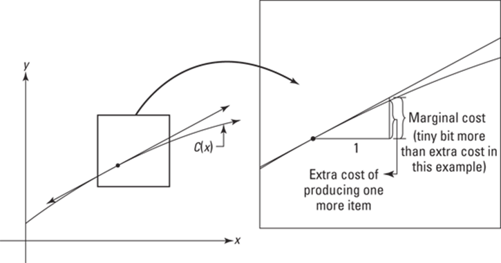
FIGURE 13-5: The graph of a cost function ![]()
Look at the blown-up square on the right in the figure. The derivative of ![]() at the point of tangency gives you the slope of the tangent line and thus the amount you go up as you go 1 to the right along the tangent line. (This amount is labeled in the figure as marginal cost.) Going 1 to the right along the cost function itself shows you the increase in cost of producing one more item. (This is labeled as the extra cost.) Because the tangent line is a good approximation of the cost function, the derivative of C — called the marginal cost — is the approximate increase in cost of producing one more item. Marginal revenue and marginal profit work the same way.
at the point of tangency gives you the slope of the tangent line and thus the amount you go up as you go 1 to the right along the tangent line. (This amount is labeled in the figure as marginal cost.) Going 1 to the right along the cost function itself shows you the increase in cost of producing one more item. (This is labeled as the extra cost.) Because the tangent line is a good approximation of the cost function, the derivative of C — called the marginal cost — is the approximate increase in cost of producing one more item. Marginal revenue and marginal profit work the same way.
Definition of marginal cost, marginal revenue, and marginal profit:
· Marginal cost equals the derivative of the cost function.
· Marginal revenue equals the derivative of the revenue function.
· Marginal profit equals the derivative of the profit function.
Before doing an example involving marginals, there’s one more piece of business to take care of. A demand function tells you how many items will be purchased (what the demand will be) given the price. The lower the price, of course, the higher the demand; and the higher the price, the lower the demand. You’d think that the number purchased should be a function of the price — input a price and find out how many items people will buy at that price — but traditionally, a demand function is written the other way around. The price is expressed as a function of the number demanded. I know that seems a bit odd, but don’t sweat it — the function works either way. Think of it like this: If a retailer wants to sell a given number of items, the demand function tells the retailer what he or she should set the selling price at.
Okay, so here’s the example. A widget manufacturer determines that the demand function for his widgets is
![]()
where p is the price of a widget and x is the number of widgets demanded. The cost of producing x widgets is given by the following cost function:
![]()
Determine the marginal cost, marginal revenue, and marginal profit at ![]() widgets. Also, how many widgets should be manufactured, and what should they be sold for to produce the maximum profit, and what is that maximum profit? (If you get through all this, I’ll nominate you for the Nobel Prize in Economics.)
widgets. Also, how many widgets should be manufactured, and what should they be sold for to produce the maximum profit, and what is that maximum profit? (If you get through all this, I’ll nominate you for the Nobel Prize in Economics.)
Marginal cost
Marginal cost is the derivative of the cost function, so take the derivative and evaluate it at ![]() :
:
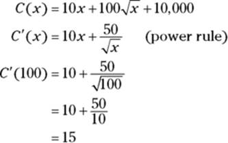
Thus, the marginal cost at ![]() is $15 — this is the approximate cost of producing the 101st widget.
is $15 — this is the approximate cost of producing the 101st widget.
Marginal revenue
Revenue, ![]() , equals the number of items sold, x, times the price, p:
, equals the number of items sold, x, times the price, p:
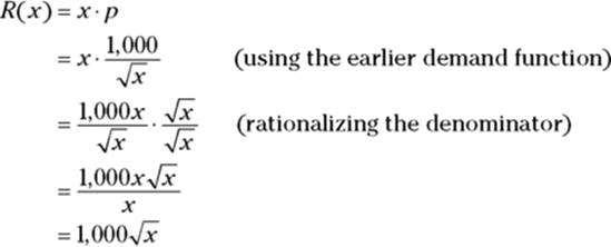
Marginal revenue is the derivative of the revenue function, so take the derivative of ![]() and evaluate it at
and evaluate it at ![]() :
:
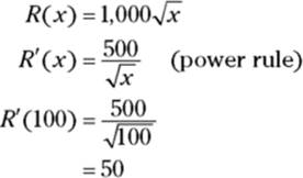
Thus, the approximate revenue from selling the 101st widget is $50.
Marginal profit
Profit, ![]() , equals revenue minus cost. So,
, equals revenue minus cost. So,
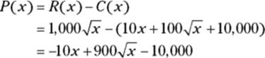
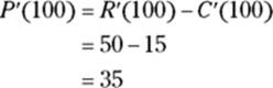
Marginal profit is the derivative of the profit function, so take the derivative of ![]() , and evaluate it at
, and evaluate it at ![]() :
:
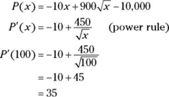
Selling the 101st widget brings in an approximate profit of $35.
Marginal profit short cuts: Did you notice either of the two shortcuts you could have taken here? First, you can use the fact that
![]()
to determine ![]() directly, without first determining
directly, without first determining ![]() . Then, after getting
. Then, after getting ![]() , you just plug 100 into x for your answer.
, you just plug 100 into x for your answer.
And, if all you want to know is ![]() , you can use the following really short shortcut:
, you can use the following really short shortcut:
This is common sense. If it costs you about $15 to produce the 101st widget and you sell it for about $50, then your profit is about $35.
I did it the long way because you need both the profit function, ![]() , and the marginal profit function,
, and the marginal profit function, ![]() , for the problems below.
, for the problems below.
Maximum profit
To determine maximum profit, set the derivative of profit — that’s marginal profit — equal to zero, solve for x, and then plug the result into the profit function:
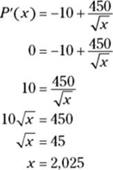
So, maximum profit occurs when 2,025 widgets are sold. Plug this into ![]() :
:
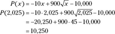
Thus, the maximum profit is $10,250. (Extra credit: Did you see where I got a bit lazy here? The derivative of the profit function is zero at x = 2,025, but that doesn’t guarantee that there’s a max at that x-value. There could instead be a min or an inflection point there. You could use either the first or second derivative test (see Chapter 11) to show that it’s actually a max. But I just peaked at a graph of the profit function and saw that it’s sort of an upside-down cup shape, so I knew that there was a max at the top of the cup at x = 2,025.)
Finally, plug the number sold into the demand function to determine the profit-maximizing price:
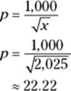
So, the maximum profit of $10,250 occurs when the price is set at $22.22. At this price, 2,025 widgets will be sold. Figure 13-6 sums up these results. Note that because profit equals revenue minus cost, the vertical distance or gap between the revenue and cost functions at a given x-value gives the profit at that x-value. Maximum profit occurs where the gap is greatest.
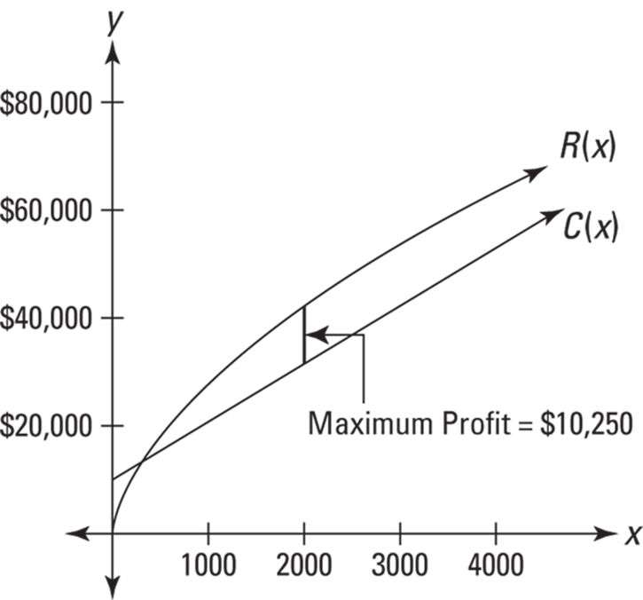
FIGURE 13-6: The revenue and cost functions. The vertical distance between them, at a given x-value, represents the profit.
(Note that although the scale of this graph makes ![]() look like a straight line, its middle term of
look like a straight line, its middle term of ![]() means that it is not exactly straight.)
means that it is not exactly straight.)
And here’s another thing. Because maximum profit occurs where ![]() , and because
, and because ![]() , it follows that the profit will be greatest where
, it follows that the profit will be greatest where ![]() — in other words, where
— in other words, where ![]() . And when
. And when ![]() the slopes of the functions’ tangent lines are equal. So, if you were to draw tangent lines to
the slopes of the functions’ tangent lines are equal. So, if you were to draw tangent lines to ![]() and
and ![]() where the gap between the two is greatest, these tangents would be parallel. Right about now you’re probably thinking something like — Such symmetry, such simple elegance, such beauty! Verily, the mathematics muse seduces the heart as much as the mind. Yeah, it’s nice all right, but let’s not get carried away.
where the gap between the two is greatest, these tangents would be parallel. Right about now you’re probably thinking something like — Such symmetry, such simple elegance, such beauty! Verily, the mathematics muse seduces the heart as much as the mind. Yeah, it’s nice all right, but let’s not get carried away.