Calculus For Dummies, 2nd Edition (2014)

Part V. Integration and Infinite Series

Chapter 17. Forget Dr. Phil: Use the Integral to Solve Problems

IN THIS CHAPTER

One mean theorem: “Random acts of kindness!? Don’t make me laugh.”

Adding up the area between curves

Figuring out volumes of odd shapes with the deli meat method

Mastering the disk and washer methods

Finding arc length and surface area

As I say in Chapter 14, integration is basically just adding up small pieces of something to get the total for the whole thing — really small pieces, actually, infinitely small pieces. Thus, the integral

tells you to add up all the little pieces of distance traveled during the 15-second interval from 5 to 20 seconds to get the total distance traveled during that interval.

In all problems, the little piece after the integration symbol is always an expression in x (or some other variable). For the above integral, for instance, the little piece of distance might be given by, say, , Then the definite integral

would give you the total distance traveled. Because you’re now an expert at computing integrals like the one immediately above, that’s no longer the issue; your main challenge in this chapter is simply to come up with the algebraic expression for the little pieces you’re adding up. But before we begin the adding-up problems, I want to cover a couple other integration topics: mean value and average value.

The Mean Value Theorem for Integrals and Average Value

The best way to understand the mean value theorem for integrals is with a diagram — look at Figure 17-1.

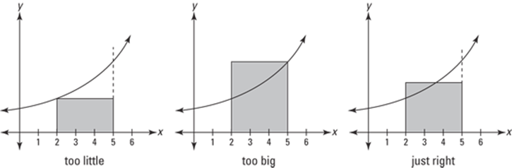
FIGURE 17-1: A visual “proof” of the mean value theorem for integrals.

The graph on the left in Figure 17-1 shows a rectangle whose area is clearly less than the area under the curve between 2 and 5. This rectangle has a height equal to the lowest point on the curve in the interval from 2 to 5. The middle graph shows a rectangle whose height equals the highest point on the curve. Its area is clearly greater than the area under the curve. By now you’re thinking, “Isn’t there a rectangle taller than the short one and shorter than the tall one whose area is the same as the area under the curve?” Of course. And this rectangle obviously crosses the curve somewhere in the interval. This so-called “mean value rectangle,” shown on the right, basically sums up the mean value theorem for integrals. It’s really just common sense. But here’s the mumbo jumbo.

The mean value theorem for integrals: If is a continuous function on the closed interval , then there exists a number c in the closed interval such that

The theorem basically just guarantees the existence of the mean value rectangle. (Note that there can only be one mean value rectangle, but its top will sometimes cross the function more than once. Thus, there can be more than one c value that satisfies the theorem.)

The area of the mean value rectangle — which is the same as the area under the curve — equals length times width, or base times height, right? So, if you divide its area, by its base, , you get its height, . This height is the average value of the function over the interval in question.

Average value: The average value of a function over a closed interval is

which is the height of the mean value rectangle.

Here’s an example. What’s the average speed of a car between seconds and seconds whose speed in feet per second is given by the function ? The definition of average value gives you the answer in one step: the average speed is . Evaluate that integral and you’re done. (That’s all there is to it, so the two-step process below is somewhat superfluous. However, it shows the logic underlying the average value idea.)

1. Determine the area under the curve between 9 and 16.

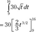
This area, by the way, is the total distance traveled during the period from 9 to 16 seconds, namely 740 feet. Do you see why? Consider the mean value rectangle for this problem. Its height is a speed (because the function values, or heights, are speeds) and its base is an amount of time, so its area is speed times time which equals distance. Alternatively, recall that the derivative of position is velocity (see Chapter 12). So, the antiderivative of velocity — what I just did in this step — is position, and the change of position from 9 to 16 seconds gives the total distance traveled.

2. Divide this area, total distance, by the time interval from 9 to 16, namely 7.

The definition of average value tells you to multiply the total area by , which in this problem is . But because dividing by 7 is the same as multiplying by , you can divide like I do in this step. It makes more sense to think about these problems in terms of division: area equals base times height, so the height of the mean value rectangle equals its area divided by its base.

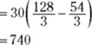
THE MVT FOR INTEGRALS AND FOR DERIVATIVES: TWO PEAS IN A POD

Remember the mean value theorem for derivatives from Chapter 11? The graph on the left in the figure shows how it works for the function . The basic idea is that there’s a point on the curve between 0 and 2 where the slope is the same as the slope of the secant line from to — that’s a slope of 4. When you do the math, you get for this point. Well, it turns out that the point guaranteed by the mean value theorem for integrals — the point where the mean value rectangle crosses the derivative of this curve (shown on the right in the figure) — has the very same x-value. Pretty nice, eh?

If you really want to understand the intimate relationship between differentiation and integration, think long and hard about the many connections between the two graphs in the accompanying figure. This figure is a real gem, if I do say so myself. (For more on the differentiation/integration connection, check out my other favorites, Figures 15-9 and 15-10.)

The Area between Two Curves — Double the Fun

This is the first of several topics in this chapter where your task is to come up with an expression for a little bit of something, then add up the bits by integrating. For this first problem type, the little bit is a narrow rectangle that sits on one curve and goes up to another. Here’s an example: Find the area between and from to . See Figure 17-2.

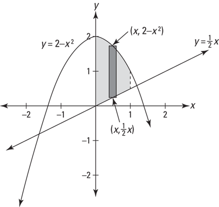
FIGURE 17-2: The area between and from to .

To get the height of the representative rectangle in Figure 17-2, subtract the y-coordinate of its bottom from the y-coordinate of its top — that’s . Its base is the infinitesimal dx. So, because area equals height times base,

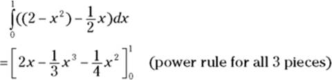
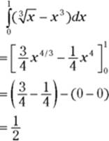
Now you just add up the areas of all the rectangles from 0 to 1 by integrating:

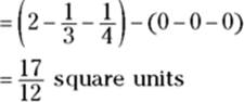
Now to make things a little more twisted, in the next problem the curves cross (see Figure 17-3). When this happens, you have to split the total shaded area into two separate regions before integrating. Try this one: Find the area between and from to .

FIGURE 17-3: Who’s on top?

1. Determine where the curves cross.

They cross at , so you’ve got two separate regions: one from 0 to 1 and another from 1 to 2.

2. Figure the area of the region on the left.

For this region, is above . So the height of a representative rectangle is , its area is height times base, or , and the area of the region is, therefore,

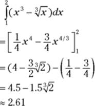
3. Figure the area of the region on the right.

In the right-side region, is above , so the height of a rectangle is and thus you’ve got

4. Add up the areas of the two regions to get the total area.

Height equals top minus bottom. Note that the height of a representative rectangle is always its top minus its bottom, regardless of whether these numbers are positive or negative. For instance, a rectangle that goes from 20 up to 30 has a height of , or 10; a rectangle that goes from up to 8 has a height of , or 11; and a rectangle that goes from up to has a height of , or 5.

If you think about this top-minus-bottom method for figuring the height of a rectangle, you can now see — assuming you didn’t already see it — why the definite integral of a function counts area below the x-axis as negative. (I mention this in Chapters 14 and 15.) For example, consider Figure 17-4.

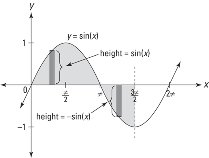
FIGURE 17-4: What’s the shaded area? Hint: it’s not

If you want the total area of the shaded region shown in Figure 17-4, you have to divide the shaded region into two separate pieces like you did in the last problem. One piece goes from 0 to , and the other from to .

For the first piece, from 0 to , a representative rectangle has a height equal to the function itself, , because its top is on the function and its bottom is at zero — and of course, anything minus zero is itself. So the area of this first piece is given by the ordinary definite integral .

But for the second piece from to , the top of a representative rectangle is at zero — recall that the x-axis is the line — and its bottom is on , so its height is , or just . So, to get the area of this second piece, you figure the definite integral of the negative of the function, , which is the same as    .

Because this negative integral gives you the ordinary, positive area of the piece below the x-axis, the positive definite integral gives a negative area. That’s why if you figure the definite integral over the entire span, the piece below the x-axis counts as a negative area, and the answer gives you the net of the area above the x-axis minus the area below the axis — rather than the total shaded area.

Finding the Volumes of Weird Solids

In geometry, you learned how to figure the volumes of simple solids like boxes, cylinders, and spheres. Integration enables you to calculate the volumes of an endless variety of much more complicated shapes.

The meat-slicer method

This metaphor is actually quite accurate. Picture a hunk of meat being cut into very thin slices on one of those deli meat slicers. That’s the basic idea here. You slice up a three-dimensional shape, then add up the volumes of the slices to determine the total volume.

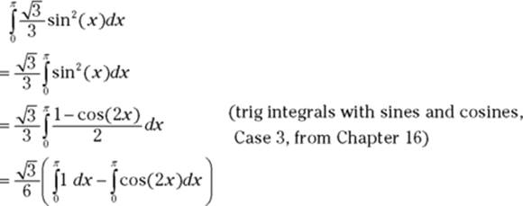
Here’s a problem: What’s the volume of the solid whose length runs along the x-axis from 0 to and whose cross sections perpendicular to the x-axis are equilateral triangles such that the midpoints of their bases lie on the x-axis and their top vertices are on the curve ? Is that a mouthful or what? This problem is almost harder to describe and to picture than it is to do. Take a look at this thing in Figure 17-5.

FIGURE 17-5: One weird hunk of pastrami.

So what’s the volume?

1. Determine the area of any old cross section.

Each cross section is an equilateral triangle with a height of . (The height of the second triangle from the left is shown in the figure.) If you do the geometry, you’ll see that the base of each triangle is times its height, or . (Hint: Half of an equilateral triangle is a 30°-60°-90° triangle.) So, the triangle’s area, given by is , or .

2. Find the volume of a representative slice.

The volume of a slice is just its cross-sectional area times its infinitesimal thickness, dx. So you’ve got the volume:

3. Add up the volumes of the slices from 0 to by integrating.

If the following seems a bit difficult, well, heck, you better get used to it. This is calculus after all. (Actually, it’s not really that bad if you go through it patiently, step by step.)

It’s a piece o’ cake slice o’ meat.

The disk method

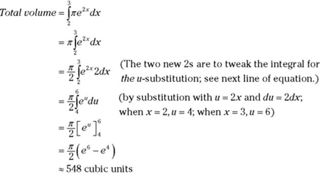
This technique is basically the same as the meat slicer method — actually it’s a special case of the meat slicer method that you use when the cross-sections are all circles. Here’s how it works. Find the volume of the solid — between and — generated by rotating the curve about the x-axis. See Figure 17-6.

1. Determine the area of any old cross section.

Each cross section is a circle with radius . So, its area is given by the formula for the area of a circle, . Plugging into r gives you

2. Tack on dx to get the volume of an infinitely thin representative disk.

3. Add up the volumes of the disks from 2 to 3 by integrating.

A representative disk is located at no particular place. Note that Step 1 refers to “any old” cross section. I call it that because when you consider a representative disk like the one shown in Figure 17-6, you should focus on a disk that’s in no place in particular. The one shown in Figure 17-6 is located at an unknown position on the x-axis, and its radius goes from the x-axis up to the curve . Thus, its radius is the unknownlength of . If, instead, you use some special disk like the left-most disk at , you’re more likely to make the mistake of thinking that a representative disk has some known radius like . (This tip also applies to the meat-slicer method in the previous section and the washer method in the next section.)

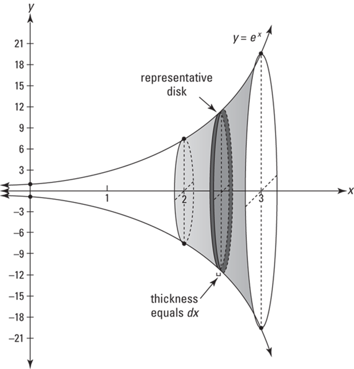
FIGURE 17-6: A sideways stack of disks.

The Washer Method

The only difference between the washer method and the disk method is that now each slice has a hole in its middle that you have to subtract. There’s nothing to it.

Here you go. Take the area bounded by and , and generate a solid by revolving that area about the x-axis. See Figure 17-7.

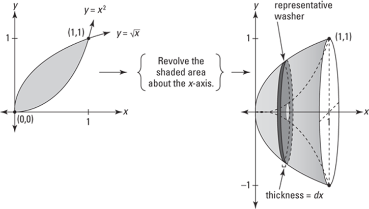
FIGURE 17-7: A sideways stack of washers — just add up the volumes of all the washers.

Just think: All the forces of the evolving universe and all the twists and turns of your life have brought you to this moment when you are finally able to calculate the volume of this solid — something for your diary. So what’s the volume of this bowl-like shape?

1. Determine where the two curves intersect.

It should take very little trial and error to see that and intersect at and — how nice is that? So the solid in question spans the interval on the x-axis from 0 to 1.

2. Figure the cross-sectional area of a thin representative washer.

Each slice has the shape of a washer — see Figure 17-8 — so its cross-sectional area equals the area of the entire circle minus the area of the hole.

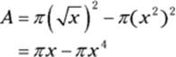
The area of the circle minus the hole is , where R is the outer radius (the big radius) and r is the hole’s radius (the little radius). For this problem, the outer radius is and the hole’s radius is , giving you

3. Multiply this area by the thickness, dx, to get the volume of a representative washer.

4. Add up the volumes of the even-thinner-than-paper-thin washers from 0 to 1 by integrating.

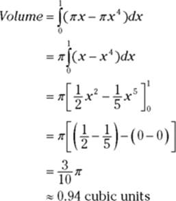
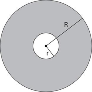
FIGURE 17-8: The shaded area equals The whole minus the hole — get it?

Area equals big circle minus little circle. Focus on the simple fact that the area of a washer is the area of the entire disk, , minus the area of the hole, : Thus, . When you integrate, you get . If you factor out the pi, and bring it to the outside of the integral, you get which is the formula given in most books. But if you just learn that formula by rote, you may forget it. You’re more likely to remember the formula and how to do these problems if you understand the simple big-circle-minus-little-circle idea.

The matryoshka-doll method

Another method for calculating volume (which may not be covered in your calculus course) is the cylindrical shell method. Instead of cutting up the volume in question into slices, disks, or washers, you cut it up into thin concentric cylinders. The concentric cylinders fit inside each other like those nested Russian dolls. For an example of one of these problems, check out my online article on the matryoshka doll method at www.dummies.com/go/calculus/.

Analyzing Arc Length

So far in this chapter, you’ve added up the areas of thin rectangles to get total area and the volumes of thin slices to get total volume. Now, you’re going to add up minute lengths along a curve to get the whole length.

I could just give you the formula for arc length (the length along a curve), but I’d rather show you why it works and how to derive it. Lucky you. The idea is to divide a length of curve into tiny sections, figure the length of each section, and then add up all the lengths. Figure 17-9 shows how each section of a curve can be approximated by the hypotenuse of a tiny right triangle.

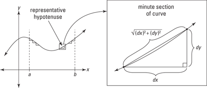
FIGURE 17-9: The Pythagorean theorem, is the key to the arc length formula.

You can imagine that as you zoom in further and further, dividing the curve into more and more sections, the minute sections of the curve get straighter and straighter, and thus the perfectly straight hypotenuses become better and better approximations of the curve. That’s why — when this process of adding up smaller and smaller sections is taken to the limit — you get the precise length of the curve.

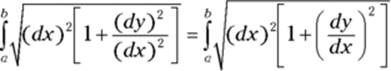
So, all you have to do is add up all the hypotenuses along the curve between your start and finish points. The lengths of the legs of each infinitesimal triangle are dx and dy, and thus the length of the hypotenuse — given by the Pythagorean theorem — is

To add up all the hypotenuses from a to b along the curve, you just integrate:

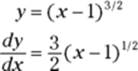
A little tweaking and you have the formula for arc length. First, factor out a under the square root and simplify:

Now you can take the square root of — that’s dx, of course — and bring it outside the radical, and, voilà, you’ve got the formula.

Arc length formula: The arc length along a curve, , from a to b, is given by the following integral:

The expression inside this integral is simply the length of a representative hypotenuse.

Try this one: What’s the length along from to ?

1. Take the derivative of your function.

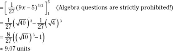
2. Plug this into the formula and integrate.

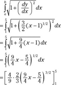
(See how I got that? It’s the guess-and-check integration technique with the reverse power rule. The is the tweak amount you need because of the coefficient .)

Now if you ever find yourself on a road with the shape of and your odometer is broken, you can figure the exact length of your drive. Your friends will be very impressed — or very concerned.

Surfaces of Revolution — Pass the Bottle ’Round

A surface of revolution is a three-dimensional surface with circular cross sections, like a vase or a bell or a wine bottle. For these problems, you divide the surface into narrow circular bands, figure the surface area of a representative band, and then just add up the areas of all the bands to get the total surface area. Figure 17-10 shows such a shape with a representative band.

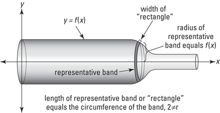
FIGURE 17-10: The wine bottle problem. If you’re sick of calculus, chill out and take a look at Wine For Dummies.

What’s the surface area of a representative band? Well, if you cut the band and unroll it, you get sort of a long, narrow rectangle whose area, of course, is length times width. The rectangle wraps around the whole circular surface, so its length is the circumference of the circular cross section, or , where r is the height of the function (for garden-variety problems anyway). The width of the rectangle or band is the same as the length of the infinitesimal hypotenuse you used in the section on arc length, namely . Thus, the surface area of a representative band, from length times width, is , which brings us to the formula.

Surface of revolution formula: A surface generated by revolving a function, about an axis has a surface area — between a and b — given by the following integral:

If the axis of revolution is the x-axis, r will equal — as shown in Figure 17-10. If the axis of revolution is some other line, like , it’s a bit more complicated — something to look forward to.

Now try one: What’s the surface area — between and — of the surface generated by revolving about the x-axis? See Figure 17-11.

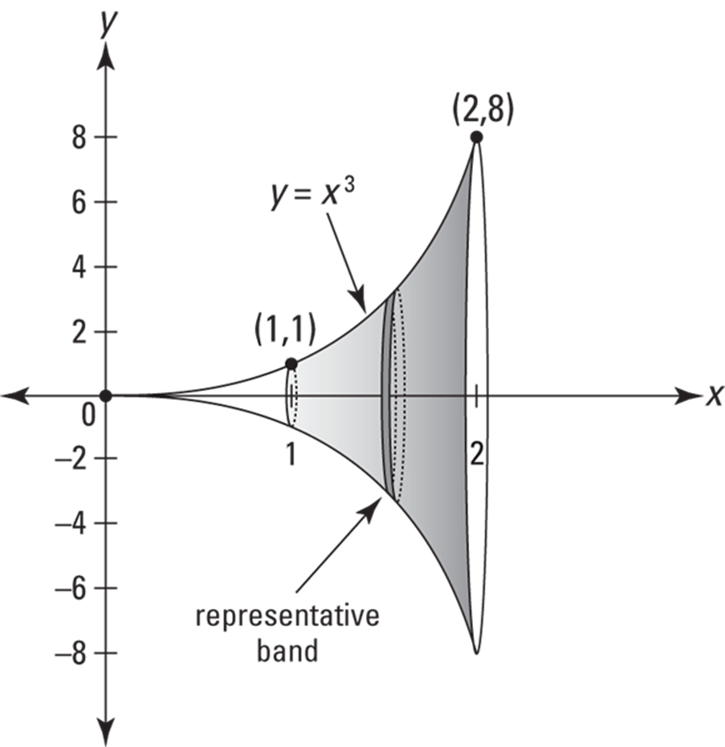
FIGURE 17-11: A surface of revolution — this one’s shaped sort of like the end of a trumpet.

1. Take the derivative of your function.

Now you can finish the problem by just plugging everything into the formula, but I’ll do it step by step to reinforce the idea that whenever you integrate, you write down a representative little bit of something — that’s the integrand — then you add up all the little bits by integrating.

2. Figure the surface area of a representative narrow band.

The radius of the band is , so its circumference is — that’s the band’s “length.” Its width, a tiny hypotenuse, is . And, thus, its area — length times width — is .

3. Add up the areas of all the bands from 1 to 2 by integrating.

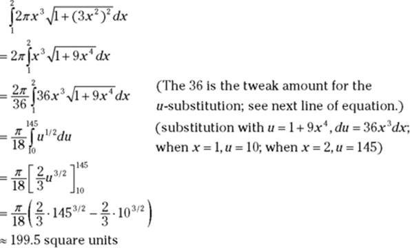
That’s a wrap.