Calculus For Dummies, 2nd Edition (2014)
Part III. Limits
IN THIS PART …
Limits: The mathematical microscope that lets you sort of zoom in on a curve to the sub-, sub-, sub-atomic level, where it becomes straight.
Limits, asymptotes, and infinity : Far out, man.
The mathematical mumbo jumbo about continuity . Plus the plain English meaning: not lifting your pencil off the paper.
Calculating limits with algebra.
Calculating limits with your calculator.
Chapter 7. Limits and Continuity
IN THIS CHAPTER
Taking a look at limits
Evaluating functions with holes — break out the mothballs
Exploring continuity and discontinuity
Limits are fundamental for both differential and integral calculus. The formal definition of a derivative involves a limit as does the definition of a definite integral. (If you’re a real go-getter and can’t wait to read the actual definitions, check out Chapters 9 and 13.) Now, it turns out that after you learn the shortcuts for calculating derivatives and integrals, you won’t need to use the longer limit methods anymore. But understanding the mathematics of limits is nonetheless important because it forms the foundation upon which the vast architecture of calculus is built (okay, so I got a bit carried away). In this chapter, I lay the groundwork for differentiation and integration by exploring limits and the closely related topic, continuity.
Take It to the Limit — NOT
Limits can be tricky. Don’t worry if you don’t grasp the concept right away.
 Informal definition of limit (the formal definition is in a few pages): The limit of a function (if it exists) for some x-value c, is the height the function gets closer and closer to as x gets closer and closer to c from the left and the right. (Note: This definition does not apply to limits where x approaches infinity or negative infinity. More about those limits later in the chapter and in Chapter 8.)
Got it? You’re kidding! Let me say it another way. A function has a limit for a given x-value c if the function zeros in on some height as x gets closer and closer to the given value c from the left and the right. Did that help? I didn’t think so. It’s much easier to understand limits through examples than through this sort of mumbo jumbo, so take a look at some.
Using three functions to illustrate the same limit
Consider the function ![]() on the left in Figure 7-1. When we say that the limit of
on the left in Figure 7-1. When we say that the limit of ![]() as x approaches 2 is 7, written as
as x approaches 2 is 7, written as ![]() , we mean that as x gets closer and closer to 2 from the left and the right,
, we mean that as x gets closer and closer to 2 from the left and the right, ![]() gets closer and closer to a height of 7. By the way, as far as I know, the number 2 in this example doesn’t have a formal name, but I call it the arrow-number. The arrow-number gives you a horizontal location in the x direction. Don’t confuse it with the answer to the limit problem or simply the limit, both of which refer to a y-value or height of the function (7 in this example). Now, look at Table 7-1.
gets closer and closer to a height of 7. By the way, as far as I know, the number 2 in this example doesn’t have a formal name, but I call it the arrow-number. The arrow-number gives you a horizontal location in the x direction. Don’t confuse it with the answer to the limit problem or simply the limit, both of which refer to a y-value or height of the function (7 in this example). Now, look at Table 7-1.
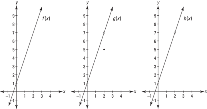
FIGURE 7-1: The graphs of the functions of f , g , and h.
TABLE 7-1 Input and Output Values of ![]() as x Approaches 2
as x Approaches 2
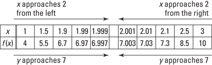
Table 7-1 shows that y is approaching 7 as x approaches 2 from both the left and the right, and thus the limit is 7. If you’re wondering what all the fuss is about — why not just plug the number 2 into x in ![]() and obtain the answer of 7 — I’m sure you’ve got a lot of company. In fact, if all functions were continuous (without gaps) like f, you could just plug in the arrow-number to get the answer, and this type of limit problem would basically be pointless. We need to use limits in calculus because of discontinuous functions like g and h that have holes.
and obtain the answer of 7 — I’m sure you’ve got a lot of company. In fact, if all functions were continuous (without gaps) like f, you could just plug in the arrow-number to get the answer, and this type of limit problem would basically be pointless. We need to use limits in calculus because of discontinuous functions like g and h that have holes.
Function g in the middle of Figure 7-1 is identical to f except for the hole at ![]() and the point at
and the point at ![]() . Actually, this function,
. Actually, this function, ![]() , would never come up in an ordinary calculus problem — I only use it to illustrate how limits work. (Keep reading. I have a bit more groundwork to lay before you see why I include it.)
, would never come up in an ordinary calculus problem — I only use it to illustrate how limits work. (Keep reading. I have a bit more groundwork to lay before you see why I include it.)
The important functions for calculus are the functions like h on the right in Figure 7-1, which come up frequently in the study of derivatives. This third function is identical to ![]() except that the point
except that the point ![]() has been plucked out, leaving a hole at
has been plucked out, leaving a hole at ![]() and no other point where x equals 2.
and no other point where x equals 2.
Imagine what the table of input and output values would look like for ![]() and
and ![]() . Can you see that the values would be identical to the values in Table 7-1 for
. Can you see that the values would be identical to the values in Table 7-1 for ![]() ? For both g and h, as x gets closer and closer to 2 from the left and the right, y gets closer and closer to a height of 7. For all three functions, the limit as x approaches 2 is 7.
? For both g and h, as x gets closer and closer to 2 from the left and the right, y gets closer and closer to a height of 7. For all three functions, the limit as x approaches 2 is 7.
This brings us to a critical point: When determining the limit of a function as x approaches, say, 2, the value of ![]() — or even whether
— or even whether ![]() exists at all — is totally irrelevant. Take a look at all three functions again where
exists at all — is totally irrelevant. Take a look at all three functions again where ![]() equals 7,
equals 7, ![]() is 5, and
is 5, and ![]() doesn’t exist (or, as mathematicians say, it’s undefined). But, again, those three results are irrelevant and don’t affect the answer to the limit problem.
doesn’t exist (or, as mathematicians say, it’s undefined). But, again, those three results are irrelevant and don’t affect the answer to the limit problem.
You don’t get to the limit. In a limit problem, x gets closer and closer to the arrow-number c, but technically never gets there, and what happens to the function when x equals the arrow-number c has no effect on the answer to the limit problem (though for continuous functions like ![]() the function value equals the limit answer and it can thus be used to compute the limit answer).
the function value equals the limit answer and it can thus be used to compute the limit answer).
Sidling up to one-sided limits
One-sided limits work like regular, two-sided limits except that x approaches the arrow-number c from just the left or just the right. The most important purpose for such limits is that they’re used in the formal definition of a regular limit (see the next section on the formal definition of a limit).
To indicate a one-sided limit, you put a little superscript subtraction sign on the arrow-number when x approaches the arrow-number from the left or a superscript addition sign when x approaches the arrow-number from the right. Like this:
![]() or
or ![]()
Look at Figure 7-2. The answer to the regular limit problem, ![]() , is that the limit does not exist because as x approaches 3 from the left and the right,
, is that the limit does not exist because as x approaches 3 from the left and the right, ![]() is not zeroing in on the same height.
is not zeroing in on the same height.
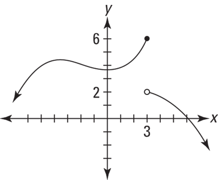
FIGURE 7-2: ![]() An illustration of two one-sided limits.
An illustration of two one-sided limits.
However, both one-sided limits do exist. As x approaches 3 from the left, ![]() zeros in on a height of 6, and when x approaches 3 from the right,
zeros in on a height of 6, and when x approaches 3 from the right, ![]() zeros in on a height of 2. As with regular limits, the value of
zeros in on a height of 2. As with regular limits, the value of ![]() has no effect on the answer to either of these one-sided limit problems. Thus,
has no effect on the answer to either of these one-sided limit problems. Thus,
![]() and
and ![]()
A function like ![]() in Figure 7-2 is called a piecewise function because it’s got separate pieces. Each part of a piecewise function has its own equation — like, for example, the following three-piece function:
in Figure 7-2 is called a piecewise function because it’s got separate pieces. Each part of a piecewise function has its own equation — like, for example, the following three-piece function:
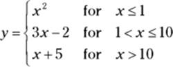
Sometimes a chunk of a piecewise function connects with its neighboring chunk, in which case the function is continuous there. And sometimes, like with ![]() , a piece does not connect with the adjacent piece — this results in a discontinuity.
, a piece does not connect with the adjacent piece — this results in a discontinuity.
The formal definition of a limit — just what you’ve been waiting for
Now that you know about one-sided limits, I can give you the formal mathematical definition of a limit. Here goes:
Formal definition of limit: Let f be a function and let c be a real number.
![]() exists if and only if
exists if and only if
1. ![]() exists,
exists,
2. ![]() exists, and
exists, and
3. ![]()
Calculus books always present this as a three-part test for the existence of a limit, but condition 3 is the only one you need to worry about because 1 and 2 are built into 3. You just have to remember that you can’t satisfy condition 3 if the left and right sides of the equation are both undefined or nonexistent; in other words, it is not true that undefined = undefined or that nonexistent = nonexistent. (I think this is why calc texts use the 3-part definition.) As long as you’ve got that straight, condition 3 is all you need to check.
When we say a limit exists, it means that the limit equals a finite number. Some limits equal infinity or negative infinity, but you nevertheless say that they do not exist. That may seem strange, but take my word for it. (More about infinite limits in the next section.)
Limits and vertical asymptotes
A rational function like ![]() has vertical asymptotes at
has vertical asymptotes at ![]() and
and ![]() . Remember asymptotes? They’re imaginary lines that the graph of a function gets closer and closer to as it goes up, down, left, or right toward infinity or negative infinity.
. Remember asymptotes? They’re imaginary lines that the graph of a function gets closer and closer to as it goes up, down, left, or right toward infinity or negative infinity. ![]() is shown in Figure 7-3.
is shown in Figure 7-3.
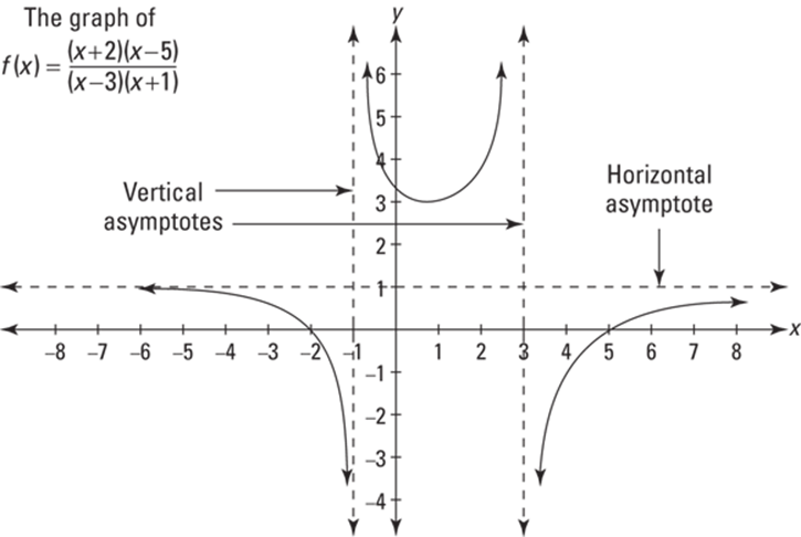
FIGURE 7-3: A typical rational function.
Consider the limit of the function in Figure 7-3 as x approaches 3. As x approaches 3 from the left, ![]() goes up to infinity, and as x approaches 3 from the right,
goes up to infinity, and as x approaches 3 from the right, ![]() goes down to negative infinity. Sometimes it’s informative to indicate this by writing,
goes down to negative infinity. Sometimes it’s informative to indicate this by writing,
![]() and
and ![]()
But it’s also correct to say that both of these limits do not exist because infinity is not a real number. And if you’re asked to determine the regular, two-sided limit, ![]() , you have no choice but to say that it does not exist because the limits from the left and from the right are unequal.
, you have no choice but to say that it does not exist because the limits from the left and from the right are unequal.
Limits and horizontal asymptotes
Up till now, I’ve been looking at limits where x approaches a regular, finite number. But x can also approach infinity or negative infinity. Limits at infinity exist when a function has a horizontal asymptote. For example, the function in Figure 7-3 has a horizontal asymptote at ![]() , which the function gets closer and closer to as it goes toward infinity to the right and negative infinity to the left. (Going left, the function crosses the horizontal asymptote at
, which the function gets closer and closer to as it goes toward infinity to the right and negative infinity to the left. (Going left, the function crosses the horizontal asymptote at ![]() and then gradually comes down toward the asymptote. Going right, the function stays below the asymptote and gradually rises up toward it.) The limits equal the height of the horizontal asymptote and are written as
and then gradually comes down toward the asymptote. Going right, the function stays below the asymptote and gradually rises up toward it.) The limits equal the height of the horizontal asymptote and are written as
![]() and
and ![]()
You see more limits at infinity in Chapter 8.
Calculating instantaneous speed with limits
If you’ve been dozing up to now, WAKE UP! The following problem, which eventually turns out to be a limit problem, brings you to the threshold of real calculus. Say you and your calculus-loving cat are hanging out one day and you decide to drop a ball out of your second-story window. Here’s the formula that tells you how far the ball has dropped after a given number of seconds (ignoring air resistance):
· ![]()
· (where h is the height the ball has fallen, in feet, and t is the amount of time since the ball was dropped, in seconds)
If you plug 1 into t, h is 16; so the ball falls 16 feet during the first second. During the first 2 seconds, it falls a total of ![]() , or 64 feet, and so on. Now, what if you wanted to determine the ball’s speed exactly 1 second after you dropped it? You can start by whipping out this trusty ol’ formula:
, or 64 feet, and so on. Now, what if you wanted to determine the ball’s speed exactly 1 second after you dropped it? You can start by whipping out this trusty ol’ formula:
![]()
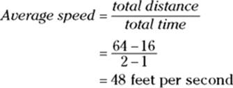
 Using the rate, or speed formula, you can easily figure out the ball’s average speed during the 2nd second of its fall. Because it dropped 16 feet after 1 second and a total of 64 feet after 2 seconds, it fell
 ![]() , or 48 feet from
, or 48 feet from ![]() second to
second to ![]() seconds. The following formula gives you the average speed:
seconds. The following formula gives you the average speed:
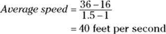
But this isn’t the answer you want because the ball falls faster and faster as it drops, and you want to know its speed exactly 1 second after you drop it. The ball speeds up between 1 and 2 seconds, so this average speed of 48 feet per second during the 2nd second is certain to be faster than the ball’s instantaneous speed at the end of the 1st second. For a better approximation, calculate the average speed between ![]() second and
second and ![]() seconds. After 1.5 seconds, the ball has fallen
seconds. After 1.5 seconds, the ball has fallen ![]() or 36 feet, so from
or 36 feet, so from ![]() to
to ![]() , it falls
, it falls ![]() , or 20 feet. Its average speed is thus
, or 20 feet. Its average speed is thus
If you continue this process for elapsed times of a quarter of a second, a tenth of a second, then a hundredth, a thousandth, and a ten-thousandth of a second, you arrive at the list of average speeds shown in Table 7-2.
TABLE 7-2 Average Speeds from 1 Second to t Seconds
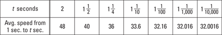
As t gets closer and closer to 1 second, the average speeds appear to get closer and closer to 32 feet per second.
Here’s the formula we used to generate the numbers in Table 7-2. It gives you the average speed between 1 second and t seconds:
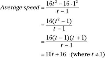
(In the line immediately above, recall that t cannot equal 1 because that would result in a zero in the denominator of the original equation. This restriction remains in effect even after you cancel the ![]() .)
.)
Figure 7-4 ![]() shows the graph of this function.
shows the graph of this function.
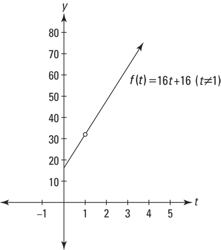
FIGURE 7-4: f(t) is the average speed between 1 second and t seconds.
This graph is identical to the graph of the line ![]() except for the hole at
except for the hole at ![]() . There’s a hole there because if you plug 1 into t in the average speed function, you get
. There’s a hole there because if you plug 1 into t in the average speed function, you get
![]()
which is undefined. And why did you get ![]() ? Because you’re trying to determine an average speed — which equals total distance divided by elapsed time — from
? Because you’re trying to determine an average speed — which equals total distance divided by elapsed time — from ![]() to
to ![]() . But from
. But from ![]() to
to ![]() is, of course, no time, and “during” this point in time, the ball doesn’t travel any distance, so you get
is, of course, no time, and “during” this point in time, the ball doesn’t travel any distance, so you get ![]() as the average speed from
as the average speed from ![]() to
to ![]() .
.
Obviously, there’s a problem here. Hold on to your hat, you’ve arrived at one of the big “Ah ha!” moments in the development of differential calculus.
Definition of instantaneous speed: Instantaneous speed is defined as the limit of the average speed as the elapsed time approaches zero.
For the falling-ball problem, you’d have
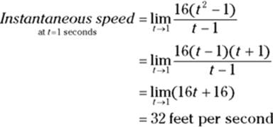
The fact that the elapsed time never gets to zero doesn’t affect the precision of the answer to this limit problem — the answer is exactly 32 feet per second, the height of the hole in Figure 7-4. What’s remarkable about limits is that they enable you to calculate the precise, instantaneous speed at a single point in time by taking the limit of a function that’s based on an elapsed time, a period between two points of time.
Linking Limits and Continuity
Before I expand on the material on limits from the earlier sections of this chapter, I want to introduce a related idea — continuity. This is such a simple concept. A continuous function is simply a function with no gaps — a function that you can draw without taking your pencil off the paper. Consider the four functions in Figure 7-5.
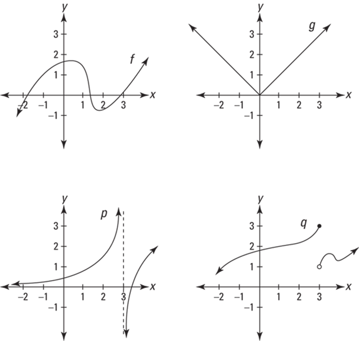
FIGURE 7-5: The graphs of the functions f, g, p, and q.
Whether or not a function is continuous is almost always obvious. The first two functions in Figure 7-5, ![]() and
and ![]() , have no gaps, so they’re continuous. The next two,
, have no gaps, so they’re continuous. The next two, ![]() and
and ![]() , have gaps at
, have gaps at ![]() , so they’re not continuous. That’s all there is to it. Well, not quite. The two functions with gaps are not continuous everywhere, but because you can draw sections of them without taking your pencil off the paper, you can say that parts of those functions are continuous. And sometimes a function is continuous everywhere it’s defined. Such a function is described as being continuous over its entire domain, which means that its gap or gaps occur at x-values where the function is undefined. The function
, so they’re not continuous. That’s all there is to it. Well, not quite. The two functions with gaps are not continuous everywhere, but because you can draw sections of them without taking your pencil off the paper, you can say that parts of those functions are continuous. And sometimes a function is continuous everywhere it’s defined. Such a function is described as being continuous over its entire domain, which means that its gap or gaps occur at x-values where the function is undefined. The function ![]() is continuous over its entire domain;
is continuous over its entire domain; ![]() , on the other hand, is not continuous over its entire domain because it’s not continuous at
, on the other hand, is not continuous over its entire domain because it’s not continuous at ![]() , which is in the function’s domain. Often, the important issue is whether a function is continuous at a particular x-value. It is unless there’s a gap there.
, which is in the function’s domain. Often, the important issue is whether a function is continuous at a particular x-value. It is unless there’s a gap there.
Continuity of polynomial functions: All polynomial functions are continuous everywhere.
Continuity of rational functions: All rational functions — a rational function is the quotient of two polynomial functions — are continuous over their entire domains. They are discontinuous at x-values not in their domains — that is, x-values where the denominator is zero.
Continuity and limits usually go hand in hand
Look at the four functions in Figure 7-5 where ![]() . Consider whether each function is continuous there and whether a limit exists at that x-value. The first two, f and g, have no gaps at
. Consider whether each function is continuous there and whether a limit exists at that x-value. The first two, f and g, have no gaps at ![]() , so they’re continuous there. Both functions also have limits at
, so they’re continuous there. Both functions also have limits at ![]() , and in both cases, the limit equals the height of the function at
, and in both cases, the limit equals the height of the function at ![]() , because as x gets closer and closer to 3 from the left and the right, y gets closer and closer to
, because as x gets closer and closer to 3 from the left and the right, y gets closer and closer to ![]() and
and ![]() , respectively.
, respectively.
Functions p and q, on the other hand, are not continuous at ![]() (or you can say that they’re discontinuous there), and neither has a regular, two-sided limit at
(or you can say that they’re discontinuous there), and neither has a regular, two-sided limit at ![]() . For both functions, the gaps at
. For both functions, the gaps at ![]() not only break the continuity, but they also cause there to be no limits there because, as you move toward
not only break the continuity, but they also cause there to be no limits there because, as you move toward ![]() from the left and the right, you do not zero in on some single y-value.
from the left and the right, you do not zero in on some single y-value.
So there you have it. If a function is continuous at an x-value, there must be a regular, two-sided limit for that x-value. And if there’s a discontinuity at an x-value, there’s no two-sided limit there … well, almost. Keep reading for the exception.
The hole exception tells the whole story
The hole exception is the only exception to the rule that continuity and limits go hand in hand, but it’s a huge exception. And, I have to admit, it’s a bit odd for me to say that continuity and limits usually go hand in hand and to talk about this exception because the exception is the whole point. When you come right down to it, the exception is more important than the rule. Consider the two functions in Figure 7-6.
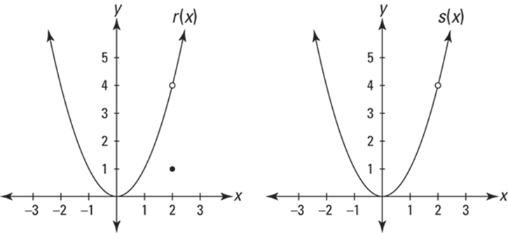
FIGURE 7-6: The graphs of the functions r and s.
These functions have gaps at ![]() and are obviously not continuous there, but they do have limits as x approaches 2. In each case, the limit equals the height of the hole.
and are obviously not continuous there, but they do have limits as x approaches 2. In each case, the limit equals the height of the hole.
The hole exception: The only way a function can have a regular, two-sided limit where it is not continuous is where the discontinuity is an infinitesimal hole in the function.
So both functions in Figure 7-6 have the same limit as x approaches 2; the limit is 4, and the facts that ![]() and that
and that ![]() is undefined are irrelevant. For both functions, as x zeros in on 2 from either side, the height of the function zeros in on the height of the hole — that’s the limit. This bears repeating, even an icon:
is undefined are irrelevant. For both functions, as x zeros in on 2 from either side, the height of the function zeros in on the height of the hole — that’s the limit. This bears repeating, even an icon:
The limit at a hole: The limit at a hole is the height of the hole.
“That’s great,” you may be thinking. “But why should I care?” Well, stick with me for just a minute. In the falling ball example in the “Calculating instantaneous speed with limits” section earlier in this chapter, I tried to calculate the average speed during zero elapsed time. This gave me ![]() . Because
. Because ![]() is undefined, the result was a hole in the function. Function holes often come about from the impossibility of dividing zero by zero. It’s these functions where the limit process is critical, and such functions are at the heart of the meaning of a derivative, and derivatives are at the heart of differential calculus.
is undefined, the result was a hole in the function. Function holes often come about from the impossibility of dividing zero by zero. It’s these functions where the limit process is critical, and such functions are at the heart of the meaning of a derivative, and derivatives are at the heart of differential calculus.
The derivative-hole connection: A derivative always involves the undefined fraction ![]() and always involves the limit of a function with a hole. (If you’re curious, all the limits in Chapter 9 — where the derivative is formally defined — are limits of functions with holes.)
and always involves the limit of a function with a hole. (If you’re curious, all the limits in Chapter 9 — where the derivative is formally defined — are limits of functions with holes.)
Sorting out the mathematical mumbo jumbo of continuity
All you need to know to fully understand the idea of continuity is that a function is continuous at some particular x-value if there is no gap there. However, because you may be tested on the following formal definition, I suppose you’ll want to know it.
Definition of continuity: A function ![]() is continuous at a point
is continuous at a point ![]() if the following three conditions are satisfied:
if the following three conditions are satisfied:
1. ![]() is defined,
is defined,
2. ![]() exists, and
exists, and
3. ![]() .
.
Just like with the formal definition of a limit, the definition of continuity is always presented as a 3-part test, but condition 3 is the only one you really need to worry about because conditions 1 and 2 are built into 3. You must remember, however, that condition 3 is not satisfied when the left and right sides of the equation are both undefined or nonexistent.
The 33333 Limit Mnemonic
Here’s a great memory device that pulls a lot of information together in one swell foop. It may seem contrived or silly, but with mnemonic devices, contrived and silly work. The 33333 limit mnemonic helps you remember five groups of three things: two groups involving limits, two involving continuity, and one about derivatives. (I realize we haven’t gotten to derivatives yet, but this is the best place to present this mnemonic. Take my word for it — nothing’s perfect.)
First, note that the word limit has five letters and that there are five 3s in this mnemonic. Next, write limit with a lower case “l” and uncross the “t” so it becomes another “l” — like this:
l i m i l
Now, the two “l”s are for limits, the two “i”s are for continuity (notice that the letter “i” has a gap in it, thus it’s not continuous), and the “m” is for slope (remember ![]() ?), which is what derivatives are all about (you’ll see that in Chapter 9 in just a few pages).
?), which is what derivatives are all about (you’ll see that in Chapter 9 in just a few pages).
Each of the five letters helps you remember three things — like this:
![]()
· 3 parts to the definition of a limit:
Look back to the definition of a limit in “The formal definition of a limit — just what you’ve been waiting for” section. Remembering that it has three parts helps you remember the parts — trust me.
· 3 cases where a limit fails to exist:
· At a vertical asymptote — called an infinite discontinuity — like at ![]() on function p in Figure 7-5.
on function p in Figure 7-5.
· At a jump discontinuity, like where ![]() on function q in Figure 7-5.
on function q in Figure 7-5.
· With a limit at infinity of an oscillating function like ![]() which goes up and down forever, never zeroing in on a single height.
which goes up and down forever, never zeroing in on a single height.
· 3 parts to the definition of continuity:
Just as with the definition of a limit, remembering that the definition of continuity has 3 parts helps you remember the 3 parts (see the section “Sorting out the mathematical mumbo jumbo of continuity”).
· 3 types of discontinuity:
· A removable discontinuity — that’s a fancy term for a hole — like the holes in functions r and s in Figure 7-6.
· An infinite discontinuity like at ![]() on function p in Figure 7-5.
on function p in Figure 7-5.
· A jump discontinuity like at ![]() on function q in Figure 7-5.
on function q in Figure 7-5.
Note that the three types of discontinuity (hole, infinite, and jump) begin with three consecutive letters of the alphabet. Since they’re consecutive, there are no gaps between h, i, and j, so they’re continuous letters. Hey, was this book worth the price or what?
· 3 cases where a derivative fails to exist:
(I explain this in Chapter 9 — keep your shirt on.)
· At any type of discontinuity.
· At a sharp point on a function, namely, at a cusp or a corner.
· At a vertical tangent (because the slope is undefined there).
Well, there you have it. Did you notice that another way this mnemonic works is that it gives you 3 cases where a limit fails to exist, 3 cases where continuity fails to exist, and 3 cases where a derivative fails to exist? Holy triple trio of nonexistence, Batman, that’s yet another 3 — the 3 topics of the mnemonic: limits, continuity, and derivatives!