Calculus For Dummies, 2nd Edition (2014)

Part III. Limits

Chapter 8. Evaluating Limits

IN THIS CHAPTER

Calculating limits with a calculator

Multiplying conjugates

Solving limits with a sandwich

Finding limits at infinity

Chapter 7 introduces the concept of a limit. This chapter gets down to the nitty-gritty and presents several techniques for calculating the answers to limits problems. And while I suspect that you were radically rapt and totally transfixed by the material in Chapter 7 — and, don’t get me wrong, that’s important stuff — it’s the problem-solving methods in this chapter that really pay the bills.

Easy Limits

A few limit problems are very easy. So easy that I don’t have to waste your time with unnecessary introductory remarks and unneeded words that take up space and do nothing to further your knowledge of the subject — instead, I can just cut to the chase and give you only the critical facts and get to the point and get down to business and … Okay, so are you ready?

Limits to memorize

You should memorize the following limits. If you fail to memorize the limits in the last three bullets, you could waste a lot of time trying to figure them out.

·

( is a horizontal line, so the limit — which is the function height — must equal c regardless of the arrow-number.)

·

·

·

·

·

·

·

Plugging and chugging

Plug-and-chug problems make up the second category of easy limits. Just plug the arrow-number into the limit function, and if the computation results in a number, that’s your answer (but see the following warning). For example,

(Don’t forget that for this method to work, the result you get after plugging in must be an ordinary number, not infinity or negative infinity or something that’s undefined.)

If you’re dealing with a function that’s continuous everywhere (like the one in the example above) or a function that’s continuous over its entire domain, this method will always work. These are well-duh limit problems, and, to be perfectly frank, there’s really no point to them. The limit is simply the function value. If you’re dealing with any other type of function, this method will only sometimes work — read on.

Beware of discontinuities. The plug-and-chug method works for any type of function, including piecewise functions, unless there’s a discontinuity at the arrow-number you plug in. In that case, if you get a number after plugging in, that number is not the limit; the limit might equal some other number or it might not exist. (See Chapter 7 for a description of piecewise functions.)

What happens when plugging in gives you a non-zero number over zero? If you plug the arrow-number into a limit like and you get any number (other than zero) divided by zero — like — then you know that the limit does not exist, in other words, the limit does not equal a finite number. (The answer might be infinity or negative infinity or just a plain old “does not exist.”)

The “Real Deal” Limit Problems

Neither of the quick methods I present in the preceding section work for most limit problems. If you plug the arrow-number into the limit expression and the result is undefined (excluding the case covered in the previous tip), you’ve got a “for real” limit problem — and a bit of work to do. This is the main focus of this section. These are the interesting limit problems, the ones that likely have infinitesimal holes, and the ones that are important for differential calculus — you see more of them in Chapter 9.

When you plug in the arrow-number and the result is undefined (often because you get ), you can try four things: your calculator, algebra, making a limit sandwich, and L’Hôpital’s rule (which is covered in Chapter 18).

Figuring a limit with your calculator

Say you want to evaluate the following limit: . The plug-and-chug method doesn’t work because plugging 5 into x produces the undefined result of , but as with most limit problems, you can solve this one on your calculator.

Note on calculators and other technology. With every passing year, there are more and more powerful calculators and more and more resources on the Internet that can do calculus for you. These technologies can give you an answer of, for example, , when the problem calls for an algebraic answer, or an answer of, for example, (not merely an approximation of 1.414), when the problem calls for a numerical answer. Older calculator models can’t give you algebraic answers, and, although they can give you exact answers to many numerical problems, they can’t give you an exact numerical answer like — and they also can’t give you an exact answer to the limit problem in the preceding paragraph.

A calculator like the TI-Nspire (or any other calculator with CAS — Computer Algebra System) can actually do that limit problem (and all sorts of much more difficult calculus problems) and give you the exact answer. The same is true of websites like Wolfram Alpha (www.wolframalpha.com).

Different calculus teachers have different policies on what technology they allow in their classes. Many do not allow the use of CAS calculators and comparable technologies because they basically do all the calculus work for you. So, the following discussion (and the rest of this book) assumes you’re using a more basic calculator (like the TI-84) without CAS capability.

Method one

The first calculator method is to test the limit function with two numbers: one slightly less than the arrow-number and one slightly more than it. So here’s what you do for the above problem, . If you have a calculator like a Texas Instruments TI-84, enter the first number, say 4.9999, on the home screen, press the Sto (store) button, then the x button, and then the Enter button (this stores the number into x). Then enter the function, , and hit Enter. The result, 9.9999, is extremely close to a round number, 10, so 10 is likely your answer. Now take a number a little more than the arrow-number, like 5.0001, and repeat the process. Since the result, 10.0001, is also very close to 10, that clinches it. The answer is 10 (almost certainly). By the way, if you’re using a different calculator model, you can likely achieve the same result with the same technique or something very close to it.

Method two

The second calculator method is to produce a table of values. Enter in your calculator’s graphing mode. Then go to “table set up” and enter the arrow-number, 5, as the “table start” number, and enter a small number, say 0.001, for — that’s the size of the x-increments in the table. Hit the Table button to produce the table. Now scroll up until you can see a couple numbers less than 5, and you should see a table of values something like the one in Table 8-1.

TABLE 8-1 TI-84 Table for After Scrolling Up to 4.998

Because y gets very close to 10 as x zeros in on 5 from above and below, 10 is the limit (almost certainly … you can’t be absolutely positive with these calculator methods, but they almost always work).

These calculator techniques are useful for a number of reasons. Your calculator can give you the answers to limit problems that are impossible to do algebraically. And it can solve limit problems that you could do with paper and pencil except that you’re stumped. Also, for problems that you do solve on paper, you can use your calculator to check your answers. And even when you choose to solve a limit algebraically — or are required to do so — it’s a good idea to create a table like Table 8-1 not just to confirm your answer, but to see how the function behaves near the arrow-number. This gives you a numerical grasp on the problem, which enhances your algebraicunderstanding of it. If you then look at the graph of the function on your calculator, you have a third, graphical or visual way of thinking about the problem.

Many calculus problems can be done algebraically, graphically, and numerically. When possible, use two or three of the approaches. Each approach gives you a different perspective on a problem and enhances your grasp of the relevant concepts.

Use the calculator methods to supplement algebraic methods, but don’t rely too much on them. First of all, the non-CAS-calculator techniques won’t allow you to deduce an exact answer unless the numbers your calculator gives you are getting close to a number you recognize — like 9.999 is close to 10, or 0.333332 is close to ; or perhaps you recognize that 1.414211 is very close to . But if the answer to a limit problem is something like , you probably won’t recognize it. The number is approximately equal to 0.288675. When you see numbers in your table close to that decimal, you won’t recognize as the limit — unless you’re an Archimedes, a Gauss, or a Ramanujan (members of the mathematics hall of fame). However, even when you don’t recognize the exact answer in such cases, you can still learn an approximate answer, in decimal form, to the limit question.

Gnarly functions may stump your calculator. The second calculator limitation is that it won’t work at all with some peculiar functions like  . This limit equals zero, but you can’t get that result with your calculator.

By the way, even when the non-CAS-calculator methods work, these calculators can do some quirky things from time to time. For example, if you’re solving a limit problem where x approaches 3, and you put numbers in your calculator that are too close to 3 (like 3.0000000001), you can get too close to the calculator’s maximum decimal length. This can result in answers that get further from the limit answer, even as you input numbers closer and closer to the arrow-number.

The moral of the story is that you should think of your calculator as one of several tools at your disposal for solving limits — not as a substitute for algebraic techniques.

Solving limit problems with algebra

You use two main algebraic techniques for “real” limit problems: factoring and conjugate multiplication. I lump other algebra techniques in the section “Miscellaneous algebra.” All algebraic methods involve the same basic idea. When substitution doesn’t work in the original function — usually because of a hole in the function — you can use algebra to manipulate the function until substitution does work (it works because your manipulation plugs the hole).

Fun with factoring

Here’s an example. Evaluate , the same problem you did with a calculator in the preceding section:

1. Try plugging 5 into x — you should always try substitution first.

You get — no good, on to plan B.

2. can be factored, so do it.

3. Cancel the from the numerator and denominator.

4. Now substitution will work.

So, , confirming the calculator answer.

By the way, the function you got after canceling the , namely , is identical to the original function, , except that the hole in the original function at has been plugged. And note that the limit as x approaches 5 is 10, which is the height of the hole at .

Conjugate multiplication — no, this has nothing to do with procreation

Try this method for fraction functions that contain square roots. Conjugate multiplication rationalizes the numerator or denominator of a fraction, which means getting rid of square roots. Try this one: Evaluate .

1. Try substitution.

Plug in 4: that gives you — time for plan B.

2. Multiply the numerator and denominator by the conjugate of , which is .

Definition of conjugate: The conjugate of a two-term expression is just the same expression with subtraction switched to addition or vice versa. The product of conjugates always equals the first term squared minus the second term squared.

Now do the rationalizing.

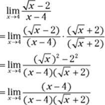
3. Cancel the from the numerator and denominator.

4. Now substitution works.

So, .

As with the factoring example, this rationalizing process plugged the hole in the original function. In this example, 4 is the arrow-number, is the limit answer, and the function has a hole at .

Miscellaneous algebra

When factoring and conjugate multiplication don’t work, try some other basic algebra, like adding or subtracting fractions, multiplying or dividing fractions, canceling, or some other form of simplification. Here’s an example: Evaluate .

1. Try substitution.

Plug in 0: That gives you — no good.

2. Simplify the complex fraction (that’s a big fraction that contains little fractions) by multiplying the numerator and denominator by the least common denominator of the little fractions, namely .

Note: You can also simplify a complex fraction by adding or subtracting the little fractions in the numerator and/or denominator, but the method described here is a bit quicker.

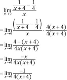
3. Now substitution works.

That’s the limit.

Take a break and make yourself a limit sandwich

When algebra doesn’t work, try making a limit sandwich. The best way to understand the sandwich or squeeze method is by looking at a graph. See Figure 8-1.

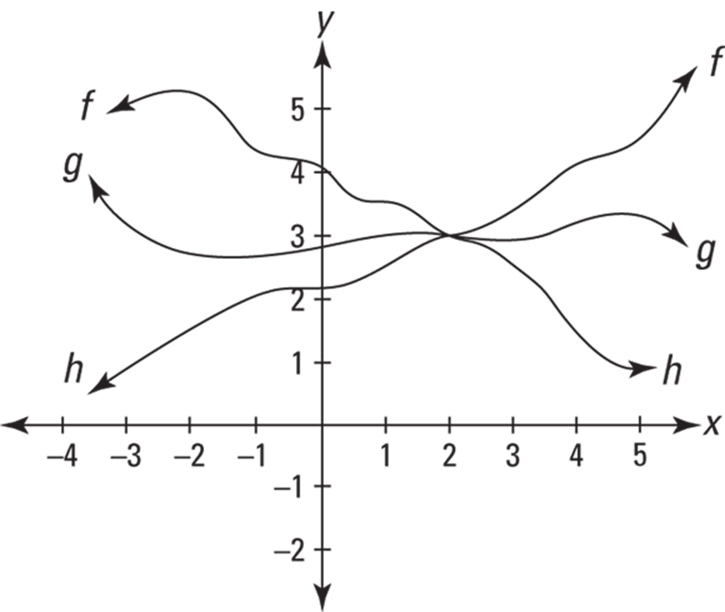
FIGURE 8-1: The sandwich method for solving a limit. Functions f and h are the bread, and g is the salami.

Look at functions f, g, and h in Figure 8-1: g is sandwiched between f and h. Since near the arrow-number of 2, f is always higher than or the same height as g, and g is always higher than or the same height as h, and since , then must have the same limit as x approaches 2 because it’s sandwiched or squeezed between f and h. The limit of both f and h as x approaches 2 is 3. So, 3 has to be the limit of g as well. It’s got nowhere else to go.

Here’s another example: Evaluate .

1. Try substitution.

Plug 0 into x. That gives you — no good, can’t divide by zero. On to plan B.

2. Try the algebraic methods or any other tricks you have up your sleeve.

Knock yourself out. You can’t do it. Plan C.

3. Try your calculator.

It’s always a good idea to see what your calculator tells you even if this is a “show your work” problem. To graph this function, set your graphing calculator’s mode to radian and the window to

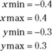
Figure 8-2 shows what the graph looks like.

It definitely looks like the limit of g is zero as x approaches zero from the left and the right. Now, check the table of values on your calculator (set TblStart to 0 and to 0.001). Table 8-2 gives some of the values from the calculator table.

These numbers sort of look like they’re getting closer and closer to zero as x gets close to zero, but they’re not convincing. This type of table doesn’t work so great for oscillating functions like sine or cosine. (Some function values on the table, for example for , are closer to zero than other values higher on the table where x is smaller. That’s the opposite of what we want to see.)

A better way of seeing that the limit of g is zero as x approaches zero is to use the first calculator method I discuss in the section “Figuring a limit with your calculator.” Enter the function on the home screen and successively plug in the x-values listed in Table 8-3 to obtain the corresponding function values. (Note: Don’t be confused: Table 8-3 is called a “table,” but it is not a table generated by a calculator’s table function. Get it?)

Now you can definitely see that g is headed toward zero.

4. Now you need to prove the limit mathematically even though you’ve already solved it on your calculator. To do this, make a limit sandwich. (Fooled you — bet you thought Step 3 was the last step.)

The hard part about using the sandwich method is coming up with the “bread” functions. (Functions f and h are the bread, and g is the salami.) There’s no automatic way of doing this. You’ve got to think about the shape of the salami function, and then use your knowledge of functions and your imagination to come up with some good prospects for the bread functions.

Because the range of the sine function is from negative 1 to positive 1, whenever you multiply a number by the sine of anything, the result either stays the same distance from zero or gets closer to zero. Thus, will never get above or below . So try graphing the functions and along with to see if f and h make adequate bread functions for g. Figure 8-3 shows that they do.

We’ve shown — though perhaps not to a mathematician’s satisfaction, egad! — that . And because , it follows that must have the same limit: voilà — .

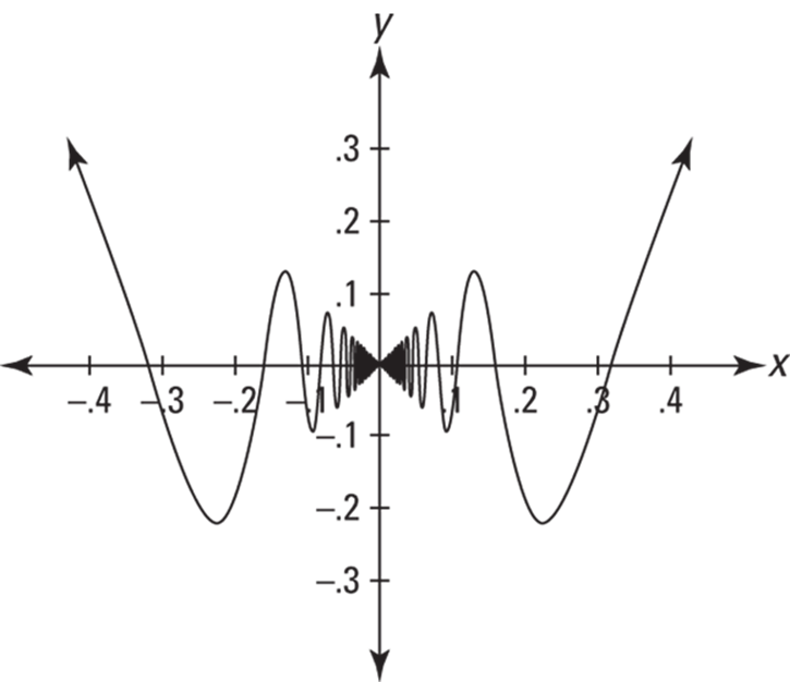
FIGURE 8-2: The graph of .

TABLE 8-2 Table of Values for

TABLE 8-3 Another Table of Values for

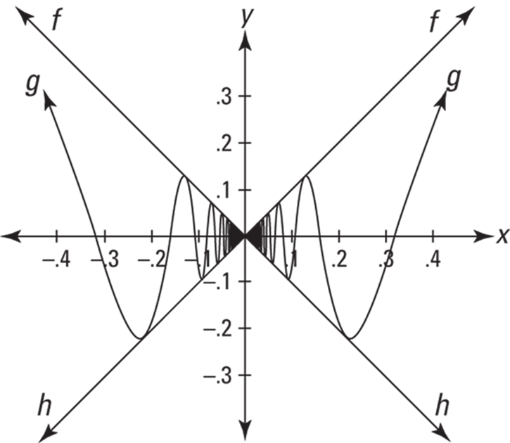
FIGURE 8-3: A graph of and . It’s a bow tie!

THE LONG AND WINDING ROAD

Consider the function shown in Figures 8-2 and 8-3 and discussed in the section about making a limit sandwich. It’s defined everywhere except at zero. If we now alter it slightly — by renaming it and then defining to be 0 — we create a new function with bizarre properties. The function is now continuous everywhere; in other words, it has no gaps. But at it seems to contradict the basic idea of continuity that says you can trace the function without taking your pencil off the paper.

Imagine starting anywhere on — which looks exactly like in Figures 8-2 and 8-3 — to the left of the y-axis and driving along the winding road toward the origin, Get this: You can start your drive as close to the origin as you like — how about the width of a proton away from — and the length of road between you and is infinitely long! That’s right. It winds up and down with such increasing frequency as you get closer and closer to that the length of your drive is actually infinite, despite the fact that each “straight-away” is getting shorter and shorter. On this long and winding road, you’ll never get to her door.

This altered function is clearly continuous at every point — with the possible exception of — because it’s a smooth, connected, winding road. And because (see the limit sandwich section for proof), and because is defined to be 0, the three-part test for continuity at 0 is satisfied. The function is thus continuous everywhere.

But tell me, how can the curve ever reach or connect to from the left (or the right)? Assuming you can traverse an infinite distance by driving infinitely fast, when you finally drive through the origin, are you on one of the up legs of the road or one of the down legs? Neither seems possible because no matter how close you are to the origin, you have an infinite number of legs and an infinite number of turns ahead of you. There is no last turn before you reach So it seems that the function can’t connect to the origin and that, therefore, it can’t be continuous there — despite the fact that the math tells us that it is.

Here’s another way of looking at it. Imagine a vertical line drawn on top of the function at . Now, keeping the line vertical, slowly slide the line to the right over the function until you pass over There are no gaps in the function, so at every instance, the vertical line crosses the function somewhere. Think about the point where the line intersects with the function. As you drag the line to the right, that point travels along the function, winding up and down along the road, and, as you drag the line over the origin, the point reaches and then passes Now tell me this: When the point hits is it on its way up or down? How can you reconcile all this? I wish I knew.

Stuff like this really messes with your mind.

Evaluating Limits at Infinity

In the previous sections, I look at limits as x approaches a finite number, but you can also have limits where x approaches infinity or negative infinity. Consider the function and check out its graph in Figure 8-4.

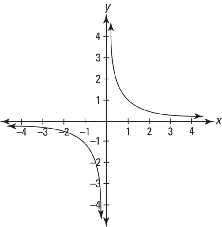
FIGURE 8-4: The graph of

You can see on the graph (in the first quadrant) that as x gets bigger and bigger — in other words, as x approaches infinity — the height of the function gets lower and lower but never gets to zero. This is confirmed by considering what happens when you plug bigger and bigger numbers into : the outputs get smaller and smaller and approach zero. This graph thus has a horizontal asymptote of (the x-axis), and we say that . The fact that x never actually reaches infinity and that f never gets to zero has no relevance. When we say that , we mean that as x gets bigger and bigger without end, f is closing in on a height of zero (or f is ultimately getting infinitely close to a height of zero). If you look at the third quadrant, you can see that the function f also approaches zero as x approaches negative infinity, which is written as .

Limits at infinity and horizontal asymptotes

Limits at infinity and horizontal asymptotes go hand in hand. Determining the limit of a function as x approaches infinity or negative infinity is the same as finding the height of the horizontal asymptote.

Let’s begin by considering rational functions. Here’s how you find the limit at infinity and negative infinity (and the height of the horizontal asymptote) of a rational function (something like ). First, note the degree of the numerator (that’s the highest power of x in the numerator) and the degree of the denominator. There are three cases:

· If the degree of the numerator is greater than the degree of the denominator, for example , there’s no horizontal asymptote, and the limit of the function as x approaches infinity (or negative infinity) does not exist (the limit will be positive or negative infinity).

· If the degree of the denominator is greater than the degree of the numerator, for example , the x-axis (that’s the line ) is the horizontal asymptote, and .

· If the degrees of the numerator and denominator are equal, take the coefficient of the highest power of x in the numerator and divide it by the coefficient of the highest power of x in the denominator. That quotient gives you the answer to the limit problem and the height of the asymptote. For example, if , , and h has a horizontal asymptote at .

Talk like a professor. To impress your friends, point your index finger upward, raise one eyebrow, and say in a professorial tone, “In a rational function where the numerator and denominator are of equal degrees, the limit of the function as x approaches infinity or negative infinity equals the quotient of the coefficients of the leading terms. A horizontal asymptote occurs at this same value.”

does not equal 1. Substitution doesn’t work for the problems in this section. If you try plugging into x in any of the rational functions in this section, you get but that does not necessarily equal 1 ( sometimes equals 1, but it often does not). A result of tells you nothing about the answer to a limit problem.

Solving limits at infinity with a calculator

Here’s a problem that can’t be done by the method in the previous section because it’s not a rational function: . But it’s a snap with a calculator. Enter the function in graphing mode, then go to table setup and set TblStart to 100,000 and to 100,000. Table 8-4 shows the results.

TABLE 8-4 Table of Values for

You can see that y is getting extremely close to 0.5 as x gets larger and larger. So 0.5 is the limit of the function as x approaches infinity, and there’s a horizontal asymptote at . If you have any doubts that the limit equals 0.5, go back to table setup and put in a humongous TblStart and , say 1,000,000,000, and check the table results again. All you see is a column of 0.5s. That’s the limit. (By the way, unlike with the rational functions in the two previous sections, the limit of this function as x approaches negative infinity doesn’t equal the limit as x approaches positive infinity: , because when you plug in you get which equals .) One more thing: Just as with regular limits, using a non-CAS (Computer Algebra System) calculator for infinite limits won’t give you an exact answer unless the numbers in the table are getting close to a number you recognize, like 0.5.

does not equal zero. Substitution does not work for the problem above, . If you plug into x, you get which does not necessarily equal zero ( sometimes equals zero, but it often does not). A result of tells you nothing about the answer to a limit problem.

Solving limits at infinity with algebra

Now try some algebra for the problem . You got the answer with a calculator, but all things being equal, it’s better to solve the problem algebraically because then you have a mathematically airtight answer. The calculator answer in this case is very convincing, but it’s not mathematically rigorous, so if you stop there, the math police may get you.

1. Try substitution — always a good idea.

No good. You get , which tells you nothing — see the Warning in the previous section. On to plan B.

Because contains a square root, the conjugate multiplication method would be a natural choice, except that that method is used for fraction functions. Well, just put over the number 1 and, voilà, you’ve got a fraction: . Now do the conjugate multiplication.

2. Multiply the numerator and denominator by the conjugate of and simplify.

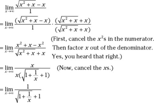
3. Now substitution works.

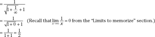
Thus, , which confirms the calculator answer.