The Calculus Primer (2011)
Part I. Functions, Rates, and Limits
Chapter 2. AVERAGE AND INSTANTANEOUS RATES
1—7. Idea of a Rate of Change. In a function, as the independent variable varies or changes by taking on one successive value after another, the value of the dependent variable also changes. But we must not confuse the value of the variable at any time with the rate at which it is changing at that time. Thus, as time goes on, the value of the public debt may be very great, but the rate at which it is changing may be comparatively small. Or, in a chemical reaction, the temperature may be relatively low, but it may be increasing very rapidly. We shall now examine the nature of a rate of change.
1—8. Constant Rate of Change. Let us consider the rate of change of a simple linear function, namely, the amount of simple interest earned by a principal of $500 at 6% per year. The graph of this function, I = (500) ![]() t, or I= 30t, is, of course, a straight line, and therefore has a constant slope. A moment’s reflection will show that if the curve representing a function is a straight line, it rises by a fixed amount in each horizontal unit interval; in this case, the constant increase is $30 per year. Thus the function I, where t is the independent variable, is increasing at a constant rate. If the interest rate were smaller, say 3%, the function I = 15t also increases at a constant, though smaller rate; the curve is again a straight line, but not as steep. Thus the rate of change is shown by the slope, or steepness, of the curve, not by its height at any point.
t, or I= 30t, is, of course, a straight line, and therefore has a constant slope. A moment’s reflection will show that if the curve representing a function is a straight line, it rises by a fixed amount in each horizontal unit interval; in this case, the constant increase is $30 per year. Thus the function I, where t is the independent variable, is increasing at a constant rate. If the interest rate were smaller, say 3%, the function I = 15t also increases at a constant, though smaller rate; the curve is again a straight line, but not as steep. Thus the rate of change is shown by the slope, or steepness, of the curve, not by its height at any point.
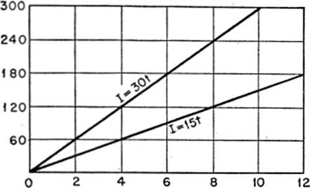
The important concept to be grasped here is that the rate of change is the amount of change in the function (or dependent variable) per unit change in the independent variable. Similarly, if the rate of change of a function is constant, the curve of the function must be a straight line, since it rises (increase in ordinate) by the same amount in each horizontal unit (increase in abscissa).
1—9. Graphic Determination of Average and Instantaneous Rates. It so happens, however, that most quantities change at a varying rate. For example, a train may cover a total distance of 150 miles in 3 hours, or at an average rate of 50 miles per hour. Yet it may well have been moving at rates greater or less than 50 miles per hour at any particular instant during those three hours, or even for the duration of some interval within that period of three hours.
It is therefore necessary to distinguish between an average rate of change during an interval, on the one hand, and an instantaneous rate at some particular instant, on the other hand.
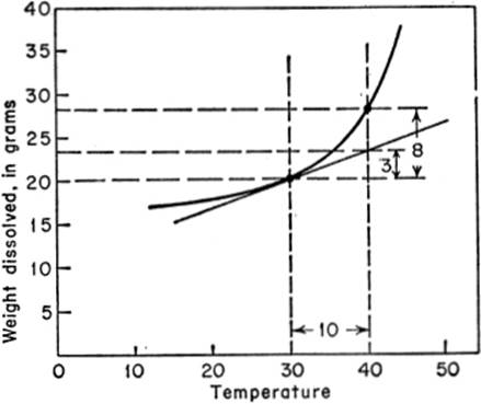
These rate of change concepts may be illustrated by the following examples. In our first illustration, the curve shows the variation of the amount of a chemical dissolved as the temperature changes. Thus, when the temperature increases from 30° to 40°, the amount dissolved increases from 20 gm. to 28 gm.; or, a total increase of 8 gm. in an interval of 10°. Thus the average rate of change equals 8 ÷ 10, or .8 gram per degree, during this 10-degree interval. Had we selected a larger or a smaller interval, or an equal interval elsewhere along the curve, the average rate of change would, of course, have been different. But now consider this question: how fast was the amount dissolved increasing at the instant when the temperature was 30°? To find the answer, we determine how steep the curve is at the point where T = 30°; that is, the tangent to the curve at this point measures the steepness of the curve at that point, and so indicates the rate at which it would continue to increase if the rate of change were to become constant at that instant Naturally, drawing a tangent to a curve at a given point “free-hand,” or by inspection, even with the aid of a ruler, is at best only an approximation. In this case, a tangent to the curve at T = 30°, when extended, meets the ordinate drawn through the abscissa T = 40° at the point where the amount is 23 gm. Hence, a uniform increaseof 3 gm. in an interval of 10°, or a constant rate of change of .3 of a gram per degree, which is the same as the instantaneous rate at the particular instant T = 30°, by virtue of the significance of the tangent at that point.
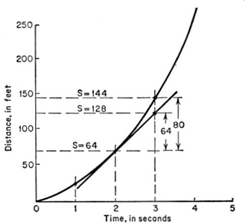
Let us take one further illustration. Consider the function s = ![]() gt2, where g = 32 ft. per sec. per sec., and s gives the distance covered by a freely falling body in t seconds. When t = 2, s = 64; when t = 3, s = 144. During the interval from t = 2 to t = 3, therefore, s increases from 64 ft. to 144 ft.; it is thus changing at an average rate of 80 ft. per sec. The tangent drawn at the point where t = 2 is found to cut the ordinate through the abscissa t = 3 at the point where s = 128; hence the instantaneous rate at t = 2 is found to be 128 − 64 = 64 ft. per sec.
gt2, where g = 32 ft. per sec. per sec., and s gives the distance covered by a freely falling body in t seconds. When t = 2, s = 64; when t = 3, s = 144. During the interval from t = 2 to t = 3, therefore, s increases from 64 ft. to 144 ft.; it is thus changing at an average rate of 80 ft. per sec. The tangent drawn at the point where t = 2 is found to cut the ordinate through the abscissa t = 3 at the point where s = 128; hence the instantaneous rate at t = 2 is found to be 128 − 64 = 64 ft. per sec.
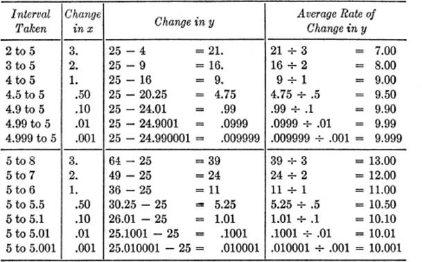
1—10. Instantaneous Rate and Very Small Intervals. To appreciate more fully the relationship of an instantaneous rate to an average rate, let us study one more illustration; for these concepts, although here presented intuitively, nevertheless lie at the very foundation of the calculus. Consider the function y = x2. Let us examine the instantaneous rate of change in the dependent variable y at the point where x = 5. We shall begin with the average rate in the interval from x = 2 to x = 5, and find the average rate as the interval taken becomes smaller and smaller. The upper half of the table shows how the average rate of change of y approaches 9.999 as the interval is taken smaller and smaller. The lower half of the table shows how the average rate of change varies as we approach the point x = 5 from the right, beginning with the interval from x = 5 to x = 8, and taking the interval smaller and smaller; the average rate of change of y now approaches 10.001. Thus the rate of change of y at the instant that x = 5 lies between 9.999 and 10.001; we shall soon learn how to compute the instantaneous rate exactly, without resorting to cumbersome graphic methods.
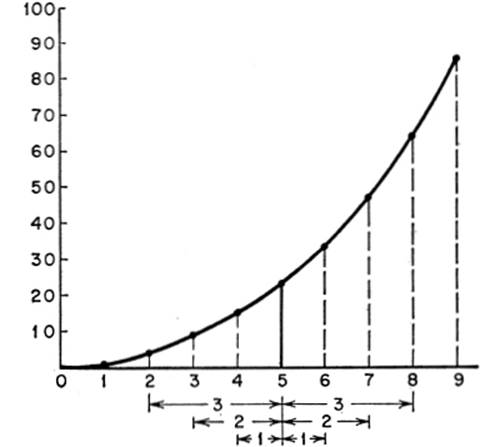
In short, the average rate of change for a very small interval is seen to be very nearly the same as the instantaneous rate at any instant during that interval, and the smaller the interval, the less the difference between the average rate and the instantaneous rate. Once more we must remind the reader not to confuse the amount of change with the rate of change. A function may increase or decrease by a very small amount in a short interval, and yet be changing very rapidly—just as a bullet may travel only a small distance in one thousandth of a second and yet be moving at a very high speed.