The Calculus Primer (2011)
Part XIV. The Definite Integral
Chapter 55. DERIVED CURVES AND INTEGRAL CURVES
14—12. Derived Curves. As we have already learned, for a curve whose equation is y = f(x), the slope of the curve at any point on the curve is given by ![]() that is, the differential coefficient of its ordinate with respect to its abscissa. If now on the same set of axes, we draw the curve whose equation is y = f′ (x), where f′ (x) represents
that is, the differential coefficient of its ordinate with respect to its abscissa. If now on the same set of axes, we draw the curve whose equation is y = f′ (x), where f′ (x) represents ![]() then at any point on this curve, the numerical measure of the ordinate is the same as that of the slope of the first curve at the point having the same abscissa. For example, if
then at any point on this curve, the numerical measure of the ordinate is the same as that of the slope of the first curve at the point having the same abscissa. For example, if
f(x) =x2 + k
and f′ (x) = 2x,
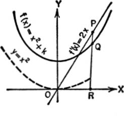
then, for any point R on the X-axis, the ordinate RQ represents the function f(x) for x = OR. The ordinate RP (where P lies on the derived curve for x = OR) is numerically equal to the slope of the original curve at Q; but the ordinate RP also represents the rate of change of the function f(x) when x = OR.
Furthermore, since
![]()
the function f(x) for x = OR is represented by the area OPR + k.
In other words: for a function f(x), if we draw the curve
y = f(x), [1]
and also its first derived curve,
y = f′(x), [2]
then the rate of change of the function for any value of x is represented not only by the slope of the first curve, but also by the ordinate of the derived curve for that value of x; and secondly, the function itself for any value of x is represented not only by the corresponding ordinate of the primary curve, but also by the area of the derived curve increased by the constant amount f(0).
The derived curve (equation [2]) is known as the curve of slopes of the first curve (equation [1]). Two such related curves are shown here. The horizontal scale is the same for both curves, but the ordinates on the primary curve represent lengths, while the ordinates on the derived curve represent tangents of angles. Thus at any point at which the primary curve has a maximum or minimum ordinate, the slope equals zero, and therefore the corresponding ordinate on the derived curve equals zero. Conversely, wherever the derived curve intersects the X-axis, the corresponding ordinate of the primary curve is a maximum or a minimum.
14—13. Integral Curves. Consider the graph of the curve
y = f(x). [1]
Let the anti-derivative of f(x) be designated by ø(x), and draw the graph of the curve
y = ![]() f (x)dx, [2]
f (x)dx, [2]
or, that is, the graph of
y = ø(x) – ø (0) = F(x). [3]
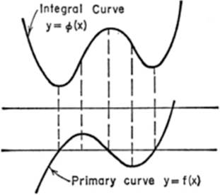
The curve y = ø(x) ø(0), or y = F(x), is known as the first integral curve of the curve [1] above. It is easily seen that
![]()
From these equations we see that the following generalizations hold:
I. For any given abscissa x, the numerical value that gives the length of the ordinate of the first integral curve is the same as the value that gives the area between the primary curve, the axes, and the ordinate for this abscissa. Hence the ordinates of the first integral curve can be used to represent the areas of the primary curve when bounded as just described.
II. For any given abscissa x, the numerical value which gives the slope of the first integral curve is the same as the value that gives the length of the ordinate of the primary curve. Hence the ordinates of the primary curve can be used to represent the slopes of the first integral curve.
EXERCISE 14—4
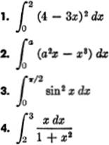
Evaluate the following:
9. Find the area of the curve y = x2 — 9 which lies below the X-axis.
10. Find the area between the equilateral hyperbola xy = 1, the ordinates at x = a, x = b, and the X-axis.
11. Find the area under one arch of the sine curve y = cos x.
12. Find the area under the semicubical parabola y2 = ax3 from the point where x = 0 to x = a.
EXERCISE 14—5
Review
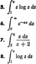
Integrate by parts:
1. ![]() ex sin x dx
ex sin x dx
2. ![]() xex dx
xex dx
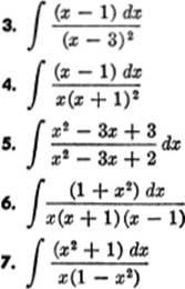
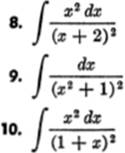
Integrate by the method of partial fractions:
Find by using the Table of Integrals, pages 371–378:
Test for convergence or divergence, and if convergent, find the interval of convergence: