The Calculus Primer (2011)
Part XV. Integration as a Process of Summation
Chapter 56. A BASIC PRINCIPLE
15—1. Two Aspects of Integration. Thus far we have regarded integration as the inverse of the operation of differentiation, and the integral was thought of as an anti-derivative. It is possible, however, to consider integration from another point of view, namely, as a process of summation, or as the addition of many similar elements. Indeed, it is largely from this point of view that the Integral Calculus developed historically, growing out of early attempts to determine the area bounded by various curves. A given area was subdivided into many small parts, and these “infinitesimal parts” were then added. The integral sign ( ![]() ) is in fact simply an elongated S, originally used as an abbreviation for “sum.” The method of summation not only throws additional light on the nature of the process of integration, but it also affords a convenient and powerful tool for solving many practical problems in science and technology to which the Integral Calculus is applied.
) is in fact simply an elongated S, originally used as an abbreviation for “sum.” The method of summation not only throws additional light on the nature of the process of integration, but it also affords a convenient and powerful tool for solving many practical problems in science and technology to which the Integral Calculus is applied.
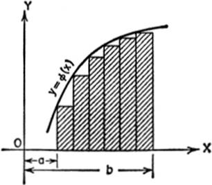
15—2. Finding an Area by Summing Up Its Component Parts. We have already seen that the area bounded by the curve y = ø(x), the X-axis, and the ordinates at x = a and x = b is given by the definite integral
![]()
but by §14—3, this may be written as
![]()
where ø(x) is the derivative of f(x). Let us suppose that the interval from x = a to x = b is divided into any number of equal subintervals, say n of them. If ordinates are erected at the points of division, and lines drawn through their extremities parallel to the X-axis, a series of rectangles will be obtained. The shaded area, consisting of the n rectangles so obtained, is an approximation to the area represented by [1] above. It will be seen that the greater the number of such subdivisions, the closer will be the approximation. If the number of rectangles is increased indefinitely, the limit of the sum of these rectangles will equal the area under the curve.
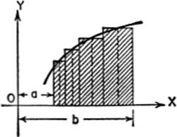
An alternative construction (which includes the above as a special case) would be the following. This time let us divide the interval from a to b into n subintervals, not necessarily equal, and erect ordinates at the points of division. Then, the sum of the rectangles constructed as shown in the figure will, as before, approximate the area under the curve; and the limit of this sum, as n → ∞, and each subinterval approaches zero, will be exactly equal to the area in question. Thus the area under a curve may be regarded as the limit of a sum.
This can be expressed analytically as shown here. Let the lengths of the successive subintervals be designated by Δx1, Δx2, Δx3, … , Δxn and the abscissas of the points chosen in the subintervals be designated by
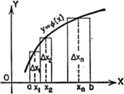
x1, x2, x3, …, xn.
Since the equation of the curve is y = ø(x), then the ordinates corresponding to x1, x2, x3, …, xn, are given by
ø(x1), ø(x2), … ø(xn).
Hence the areas of these successive rectangles are given by
ø(x1) Δx1, ø(x2) Δx2, ø(x3) Δx3, … ø(xn) Δxn
Therefore, in view of what has been said above, the area under the curve is given by
![]()
Since this area is also expressed by
![]()
we have:
![]()
15—3. The Fundamental Theorem of the Integral Calculus. Equation [2] of the preceding paragraph is, essentially, the fundamental theorem of the Integral Calculus. We restate this basic principle completely, as follows:
If ø(x) is a continuous function in the interval from x = a to x = b, and if this interval is divided into subintervals of length Δx1, Δx2, … Δxn, and if points are chosen, one in each subinterval, such that their abscissas are x1, x2, … xn, we may form the sum
![]()
then, as n approaches infinity, and each subinterval approaches zero, the limiting value of this sum is equal to the definite integral ![]()
Equation [2] may be abbreviated as follows:
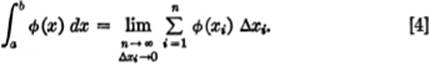
It should be noted that each term in the sum in [3], that is, each of the quantities ø(xi) Δxi, is a differential expression, inasmuch as each of the Δxi factors approaches zero as a limit. Each of these ø(xi) Δxi terms is called an elementof the total quantity (whether area, volume, pressure, etc.) whose sum is to be determined in this way.
15—4. Applying the Fundamental Theorem. The above discussion leads to the following rule of procedure to be followed when using this principle in practical problems:
I.Let the required quantity be divided into similar parts, or elements, in such a way that the limit of the sum of these parts will yield the quantity desired;
II.Express the magnitudes of these parts in such a way as to yield a sum of the form given by equation [S] above;
III.Select the appropriate limits x = a and x = b, apply the formula

and integrate.