The Calculus Primer (2011)

Part XVI. Successive and Partial Integration; Approximate Integration

Chapter 62. APPROXIMATE INTEGRATION

16—8. Need for Approximate Methods. It is frequently impossible or inconvenient to find the value of a definite integral by using the methods of integration discussed in Chapters Twelve and Thirteen. Or, it may be impossible to set up the analytical expression for the desired integration. In such cases we resort to an approximation method, of which there are several. Some approximation methods involve the use of infinite series; others are based on the measurement of an area, which may be found by computation, or by some mechanical device such as a planimeter or an integraph.

16—9. Integration by the Use of Infinite Series. When the indefinite integral of a given function f(x) dx cannot be found, it is frequently possible to expand f(x) into an ascending or descending power series in x. If this power series is convergent for a certain range of values of x, then the series obtained by integrating it term by term is also convergent within the limits for which the original power series is convergent. The more terms we take in the computation, the closer the sum will be to the value of When integrating a power series term by term within the interval of convergence, it should be remembered that neither limit of integration may be an end point of the convergence interval.

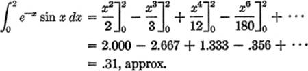
EXAMPLE 1. Find

Solution.

Multiplying (1) and (2) term by term, and combining like terms:

Series (3) is convergent for all values of x; hence, integrating (3) term by term:

Therefore:

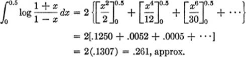
EXAMPLE 2. Find

Solution.

Subtracting (2) from (1):

Upon testing series (3) for convergence, the interval of convergence is found to be −1 < x < +1. Integrating (3):

Hence

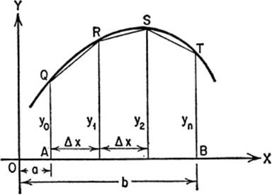
16—10. The Trapezoidal Rule. Consider the single-valued function y = f(x), and assume that it is continuous in the interval a x b. We wish to find the area under the curve from x = a to x = b. Suppose that y is positive throughout the interval from a to b. We may proceed by dividing the segment AB into n equal parts, each equal to Δx; the ordinates drawn through these points of division, y₀, y₁, y₂, · · · y_n, divide the desired area into n strips of equal width. By drawing chords QR, RS, ST, etc., we form n trapezoids, having equal altitudes (Δx), and whose bases are the successive ordinates. Now the area under the curve is approximately equal to the sum of the areas of these inscribed trapezoids. Hence

area of 1st trapezoid = Δx(y₀ + y₁);

area of 2nd trapezoid = Δx(y₁ + y₂);

area of 3rd trapezoid = Δx(y₂ + y₃);

·········································

area of nth trapezoid = Δx(y_n−1 + y_n).

By adding, we obtain

A = Δx(y₀ + 2y₁ + 2y₂ + 2y₃ + · · · + 2y_n−1 + y_n); [1]

or A = Δx(y₀ + y₁ + y₂ + · · · + y_n−1 + y_n). [2]

This is known as the Trapezoidal Rule. It may be used not only to determine an area, but also to find the approximate value of any definite integral. The greater the number of intervals taken, the more nearly will the sum of the areas of the trapezoids be equal to the area under the curve.

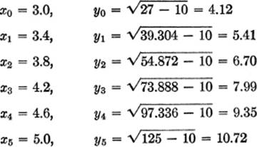
EXAMPLE 1. Find the approximate area under the curve y = from x = 3 to x = 5.

Solution. Divide the interval in question into any number of equal parts, say five parts. Thus Δx = (5 − 3) = 0.4. Hence:

Hence, substituting in formula [1] above:

A= (0.4)[4.12+2(5.41)+2(6.70)+2(7.99)+2(9.35)+10.72],

or A = (0.2) (77.22) = 154.44.

To appreciate how close the approximation can come to the exact value, consider the following example.

EXAMPLE 2. Compute the value of using the trapezoidal rule with 9 intervals; compare the result with the value obtained by direct integration.

Solution.

x₀ = 1, y₀ = (1)³ = 1

x₁ =2,y₁ = (2)³ = 8

x₂ = 3, y₂ = (3)³ = 27

······· ···················

x₉ = 10, y₉ = (10)³ = 1000

Substituting in the formula [2] for the trapezoidal rule:

A = (1)[+8+27+64+125+216+343+512+729+500],

or A = 2524, approx.

By direct integration: = (10,000 − 1) = 2499; the difference, 2524 − 2499, represents an error of less than 1%.

The trapezoidal rule may also be stated as follows:

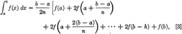
where the interval (b − a) is divided into n equal parts, and h = .

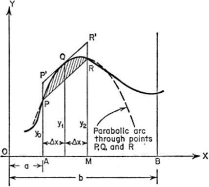
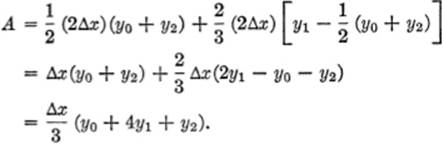
16—11. Simpson’s Rule. Also known as the parabolic rule and as the “one-third” rule, this approximation formula is obtained by dividing the interval from a to b into any even number (n) of equal sub-intervals, each equal to Δx; then, instead of drawing chords of the corresponding points on the curve to form trapezoids, we draw parabolic arcs through each successive set of three points on the curve, with the axes of these parabolas parallel to the Y-axis. We then find the area under each of these parabolic strips. The area of the first of these parabolic strips, APQRM, for example, will be: the area of trapezoid APRM + area of the parabolic segment PQR, which equals two-thirds of the area of the circumscribed parallelogram PP′R′R; hence the area of the parabolic strip equals

Similarly, the areas of the succeeding parabolic strips are given by

A = (y₂ + 4y₃ + y₄),

A = (y₄ + 4y₅ + y₆), etc.

Upon adding, we arrive at Simpson’s rule:

A = (y₀ + 4y₁ + 2y₂ + 4y₃ + 2y₄ + · · · + y_n). [4]

This may also be written, for convenience in computation, as:

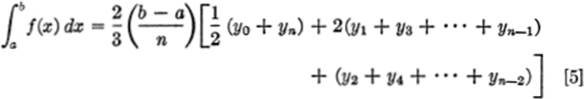
As with the trapezoidal rule, the greater the number of intervals taken; the better the approximation. For many curves, the accuracy obtained with Simpson’s rule is better than that obtained with the trapezoidal rule.

EXAMPLE. Find by Simpson’s rule, taking n = 10.

Solution.

y₀ = 9

y₁ = 16

y₂ = 25

y₃ = 36

y₄ = 49

y₅ = 64

y₆ = 81

y₇ = 100

y₈ = 121

y₉ = 144

y₁₀ = 169

Hence, by Simpson’s rule, we have:

Area = (1)[9 + 4(16) + 2(25) + 4(36) + 2(49)
+ 4(64) + 2(81) + 4(100)
+ 2(121) + 4(144) + 169]

or A = (2170) = 723.3.

NOTE. By the trapezoidal rule, A = 725.0; by direct integration, = 723.3, so that in this particular instance the use of Simpson’s rule, by coincidence, gives the exact value.

EXERCISE 16—4

1. Find by the trapezoidal rule; take n = 10. Check for accuracy by direct integration; remember that log N = (2.3026) (log₁₀ N).

2. Find by the trapezoidal rule; take n = 8; check by direct integration.

3. Find by Simpson’s rule for n = 8; check by direct integration.

4. Find by Simpson’s rule for n = 6; check by direct integration.

5. Calculate by the trapezoidal rule for 5-degree intervals. Check by direct integration; remember that Δx = 5° = .

6. Calculate taking unit intervals, by Simpson’s rule. Check by direct integration; note that log₁₀ x =

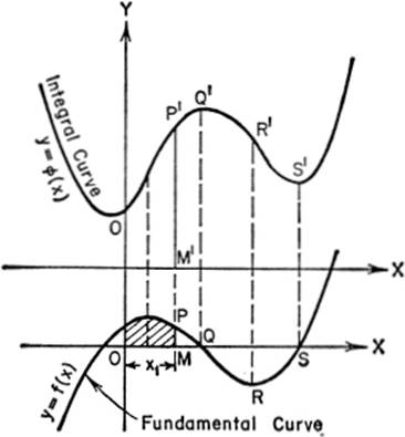
16—12. The Integraph. To find the area bounded by a curve, whether we know its equation or not, we may use a mechanical device known as the integraph. Its use depends upon the properties of integral curves, which will be briefly explained again (see §14—13).

Let ϕ(x) and f(x) be two functions related as follows:

If (1)

then the curve y = ϕ(x)(2)

is called an integral curve of the curve

y = f(x). (3)

The curve y = f(x) is called the original curve, or the fundamental curve; the curve y = ϕ(x) is more precisely known as the first integral curve, since there are also other integral curves associated with a given original curve.

This relation may also be expressed:

From the figure, it will be noted that:

(1) zero values of ordinates of the fundamental curve correspond to maximum or minimum values of ordinates of the first integral curve;

(2) maximum or minimum values of ordinates of the fundamental curve correspond to points of inflection on the first integral curve.

Since, in general, an area is given by we see that the shaded area equals but, from (4) above, we may say:

since ϕ(0) = 0, shaded area = f(x) dx = ϕ(x₁). But ϕ(x₁) = M′P′. We may therefore conclude that, for a given abscissa x₁, the number which expresses the length of the ordinate of the integral curve y = ϕ(x) is the same as the number which expresses the area between the original curve y = f(x), the axes, and the ordinate corresponding to this abscissa.

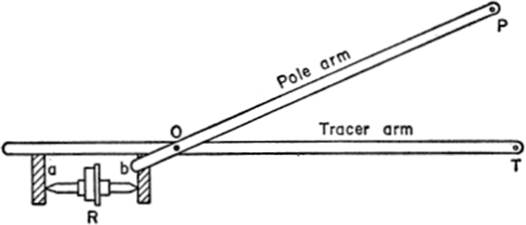
The integraph is a mechanical contrivance for drawing the first integral curve from its fundamental curve; as one movable part of a sliding framework follows the original curve, another part traces out the integral curve. Thus with the aid of this device we can find the area under, or enclosed by, a given empirical curve, simply by setting the instrument appropriately and reading the scales accurately.

16—13. The Planimeter. There are, generally speaking, three types of planimeters: the polar planimeter, the disc type, and the rolling type. The polar planimeter, for example, consists of (1) a horizontal bar OT known as the tracer arm; (2) a wheel or roller (R) of radius r turning on its axle ab; and (3) another horizontal bar OP called the pole arm. One end of the pole arm is hinged or pivoted at O, and acts as the center of rotation for the tracer arm. The other end of the pole arm (P) is known as the pole, and remains fixed throughout the operation of the planimeter; it serves as a center about which the entire instrument rotates. Any area circumscribed by the tracer point equals the product of the length of the tracer arm and the distance actually rolled over by the rim of the measuring roller.

The principle upon which the polar planimeter operates involves the calculation of the area swept over by a moving line of constant length (l). Let the area MNPN′M′QM be the area swept over by the line MN, of fixed length l; PQ and P′Q′ are two successive positions of MN, and ds the circular arc described about O by the mid-point K of PQ, as the line PQ sweeps through a differential angle dθ = angle PQOQ′P′. It can be shown that the area MN′ under consideration equals

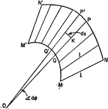
For the line PQ substitute a rod with a wheel at its center K; as the rod moves horizontally over the surface containing the area, the wheel will both roll and slide; the distance it rolls is s = 2πrn, where r = radius of the wheel and n = the number of revolutions it makes. Thus the area MN′, by substitution, equals 2πrnl.