The Calculus Primer (2011)
Part XVI. Successive and Partial Integration; Approximate Integration
Chapter 63. PRACTICAL APPLICATIONS
16—14. Statement of Principles. We shall now see how the Integral Calculus may be applied to practical problems in mechanics, physics, engineering, etc. Before studying specific illustrations, the following restatement of principles may prove helpful.
I. Integration is a process of summation. If f(x) is any function of x, the values which f(x) takes as x increases from a to b by equal increments h are: f(a), f(a + h), f(a + 2h), · · · . The limit of the sum h[f(a) + f(a + h) + f(a + 2h) + · · ·] when h = 0, or, in symbols,
![]()
is written as ![]() The process of finding this limit is known as integration.
The process of finding this limit is known as integration.
II. Integration is also a process of anti-differentiation. To find the limit of a sum of the type mentioned in (I) above, it is necessary to find a function of x, say ϕ(x), such that ![]() that is, a function ϕ(x) which when differentiated yields f(x). This process of finding an anti-derivative is also known as integration. In short, if
that is, a function ϕ(x) which when differentiated yields f(x). This process of finding an anti-derivative is also known as integration. In short, if
![]() then f(x) dx = ϕ(x) + C.
then f(x) dx = ϕ(x) + C.
III. Any definite integral may be interpreted as an area, even when the elements to be summed up represent quantities other than areas. Since ![]() is the area bounded by the curve y = f(x), the X-axis and the ordinate x = aand x = b, it follows that, even when the value of the definite integral cannot be found by the ordinary methods of integration, its approximate value can nevertheless be determined by drawing the curve y = f(x) between x = a and x = b and finding the area by approximation methods mentioned in the preceding section.
is the area bounded by the curve y = f(x), the X-axis and the ordinate x = aand x = b, it follows that, even when the value of the definite integral cannot be found by the ordinary methods of integration, its approximate value can nevertheless be determined by drawing the curve y = f(x) between x = a and x = b and finding the area by approximation methods mentioned in the preceding section.
16—15. Speed-Time-Distance Relationship. Any curve drawn to represent the speed of a moving point (or object) is known as a speed curve. Suppose that the segment AB represents the total time interval t during which the motion is considered. Let AB be divided into a large number of small, equal parts; the ordinate aA represents the speed at the beginning of the interval from a to b, and bB the speed at the end of the interval. Ordinates such as MPand NQ represent the instantaneous values of the speed at the beginnings (or ends) of the various sub-intervals.
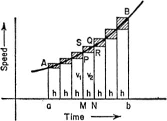
Now consider one of these sub-intervals, say MN. If the speed throughout this interval had remained the same as at the beginning of the interval, say v1, the distance covered in that interval would equal v1 × MN = the area of the rectangle MPRN, since distance = rate × time where the rate is constant. If the speed throughout the interval had been the same as that at the end of the interval, say v2, the distance covered would have been v2 × MN = the area of rectangle MSQN. The actual distance covered in the interval MN, however, lies between these two values. Similarly, if the number of intervals be increased indefinitely, the small shaded areas will decrease without limit, and the area under the curve AB bounded by aA, bB and ab will represent the actual distance covered in the interval ab. Thus the determination of distance covered when the relation between speed and time is known represents a problem in finding an area, and can be looked upon either as a problem of summation or of finding an anti-derivative.
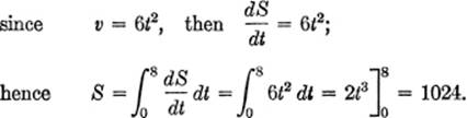
EXAMPLE 1. A body moves according to the law v = 6t2; find the distance covered in 8 seconds from rest.
Solution. First consider the problem as a summation. Let us suppose the entire interval of 8 seconds divided into n equal sub-intervals of ft seconds each, so that nh = 8, and suppose the speed to remain constant throughout each sub-interval, being equal to the speed at the beginning of each sub-interval respectively. The speeds at the beginning of successive intervals are
0, 6h2, 6(2h)2, ··· 6[(n − 1)h]2;
hence the total distance covered, on this assumption, would be
S1 = h{0 + 6h2 + 6(2h)2 + ··· + 6[(n − 1)h]2}
= 6h3[12 + 22 + 32 + · · · + (n − 1) terms],
or S1 = 6h3[![]() (n − 1)(n)(2n − 1)]. (1)
(n − 1)(n)(2n − 1)]. (1)
NOTE. In algebra it is proved that
![]()
Since nh = 8, or n = ![]() , equation (1) becomes
, equation (1) becomes
![]()
or S1 = 1024 − 192h + 8h2. (2)
Now let us assume that the speed during each sub-interval remained constant but equal to the speed at the end of each sub-interval. The total distance would then be
S2 = h[6h2 + 6(2h)2 + · · · + 6(nh)2]
= 6h3[12 + 22 + 32 + · · · to n terms]
= 6h3[![]() (n)(n + 1)(2n + 1)]
(n)(n + 1)(2n + 1)]
= h3[2n3 + 3n2 + n],
or S2 = 1024 + 192h + 8h2.(3)
The actual distance S > S1, but < S2; as h → 0, S1 → S, and S2 → S, and the limiting value S = 1024.
The same result is obtained if the problem is treated as one of finding the anti-derivative. For,
The latter method, obviously, is the more convenient when the given function can be integrated. If it cannot be integrated, we may use an approximation method for finding the area instead of the algebraic method of summation used above.
EXAMPLE 2. If a body moves so that v = 4t + 6t2, find the distance covered between the beginning of the third second and the end of the sixth second.
Solution. Here v = 4t + 6t2; hence
![]()
16—16. Force and Work. In physics we learn that when a force acts on a body, the product of the force by the distance through which it acts in the direction of the force is called the work done by the force.
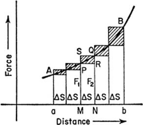
If the acting force is constant, the work done simply equals the force × displacement. But if the force is variable, we must use a method similar to the speed-time curve solution of §16—15. Now we are dealing with a force-distancecurve, such as that shown here. The ordinates represent the varying values of the force, and the intervals ab, MN, etc. represent displacements, or distances through which the body is moved by the force. Precisely the same reasoning applies here as in §16—15; thus the work done while the body suffers a displacement MN is F1 × MN = area of rectangle MPRN, or F2 × MN = rectangle MSQN, depending upon whether we assume a force of F1 or of F2 is constant. The actual total work done is ∑F·ΔS, where MN = ΔS. In general, therefore, the work done by a variable force when moving a body any distance, say x, is given by the area under a force-distance curve; or
![]()
The same result is obtained by using the anti-derivative method of reasoning. Thus, to move the body an additional distance Δx requires additional work ΔW; this equals the average force ![]() acting during Δx, multiplied by the distance Δx:
acting during Δx, multiplied by the distance Δx:
ΔW = ![]() ·Δx,
·Δx,
or ![]()
Hence the instantaneous rate at which W is increasing is
![]()
NOTE 1. In the above discussion, Δs represents any one of a large number of equal intervals, whereas the Δx-intervals need not be equal.
NOTE 2. Before integrating ![]() if F is a function of s, it must be so expressed.
if F is a function of s, it must be so expressed.
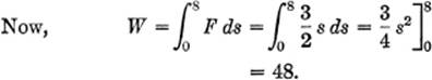
EXAMPLE 1. Find the work done in stretching a spring from its original length of 12 cm. to a length of 20 cm., if it is known that a force of 1.5 kg. will stretch it 1 cm.
Solution. Here the force varies directly as the elongation (Hooke’s Law), or F = ks, where s is the elongation; hence, since s = 1 when F = 1.5, we have 1.5 = k(1), or k = 1.5. Therefore, F = ![]() s.
s.
NOTE. Since the units used were kg. and cm., the work done equals 48 cm.-kg., 48,000 cm.-g.
EXAMPLE 2. The force (F lb.) driving a piston varies with the piston displacement (x in.) (distance moved) according to the law F = 3000/x. Find the work done from x = 8 to x = 12.
Solution.
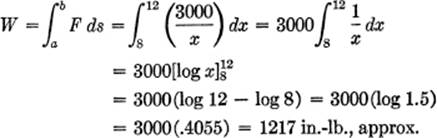
NOTE 1. When finding logarithms here, the table of natural logarithms must be used, since the relations ![]() (log x) =
(log x) = ![]() and
and ![]() = log x are based upon logarithms to the base e, not the base 10.
= log x are based upon logarithms to the base e, not the base 10.
NOTE 2. If a table of natural logarithms is not available, the value of loge N can be found from a table of common logarithms by means of the relation loge N = (2.3026) log10 N.
16—17. Liquid Pressure. From physics we know that the pressure exerted by a liquid on the walls of an open vessel is due to the head of liquid, that is, the height of liquid above that point. Hence, the pressure on any horizontalsurface simply equals the weight of the column of liquid standing on that surface as a base and having a height equal to the distance that this surface is below the free surface of the liquid. For a horizontal surface of area A at a distance h below the surface, the total pressure P is given by
P = whA,
where w = weight of liquid in pounds per cubic unit.
To find the pressure on a surface that is not horizontal, we must remember that the pressure at different points varies with the distance below the free surface, and so integration must be used. For a vertical surface, the pressure increases with the depth; the differential pressure equals the differential of the area multiplied by wh, or
dP = w·h·dA;
hence ![]()
where dA is expressed as a function of h to make integration possible, and where the limits of integration h1 and h2 are respectively the smallest and greatest heads on the surface in question.
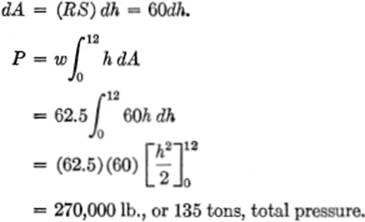
EXAMPLE 1. Find the total pressure exerted on a vertical wall of an open tank two-thirds filled with water (w = 62.5 lb./cu. ft.), if the dimensions are those given in the diagram.
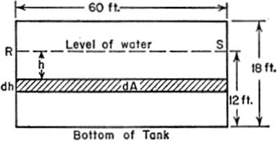
Solution. From the diagram,
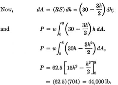
EXAMPLE 2. Find the total pressure on the vertical wall of an open tank filled with water if the wall is a trapezoid standing on the smaller base with dimensions as given.
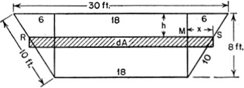
Solution. Here, to find RS, we note that if MS = x, then ![]() , or x = 6 −
, or x = 6 − ![]() .
.
Hence, RS = 18 + 2x, or RS = 30 − ![]() .
.
16—18. Center of Gravity. If we think of a plane area as divided into many small rectangles such as PQ, where the coordinates of P are (x,y), and the dimensions of the rectangle are Δx and Δy, then the area of PQ is (Δx) (Δy), and the product of the area and its distance x from the Y-axis is called the moment of PQ with respect to the Y-axis. If we sum up all such moments throughout the entire area S, we have the moment of the area with respect to the Y-axis; thus
![]()
![]()
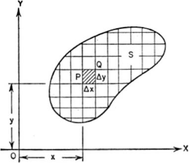
where the limits of integration are found from the equation of the boundary curve. Similarly,
![]()
Now if the moment of an area with respect to an axis is divided by the entire area, the quotient represents the average distance at which the entire area could be concentrated and still give the same moment. Let us denote these average distances by ![]() and
and ![]() ; then
; then
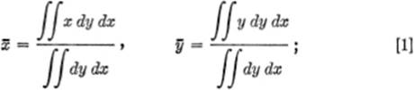
the point whose coordinates are ![]() and
and ![]() is known as the center of gravity of the area S. An alternative form of [1] is to write
is known as the center of gravity of the area S. An alternative form of [1] is to write
![]()
a form which is convenient for figures whose areas can be expressed or determined without first integrating.
EXERCISE 16—5
Review
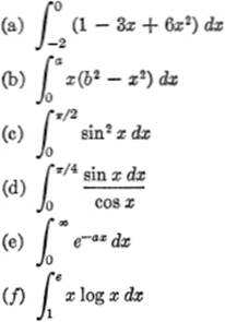
1. Evaluate the following:
2. Find the length of that part of each curve indicated:
(a) ρ = 2a sin θ, from θ = 0 to θ = π.
(b) ρ = eaθ, from ρ = 0 to ρ = 2a.
3. Find the area enclosed by the cardioid ρ = a(1 − cos θ).
4. Find the value of:
![]()
![]()
5. Find the total differential:
(a) z = ax2y3
(b) z = xy
6. If z = ![]() find:
find:
![]()
![]()
7. Determine the interval of convergence:
8. (a) Using Taylor’s theorem, prove that
![]()
(b) Using Maclaurin’s series, prove that
![]()
9. Find the following:
![]()
![]()
10. Find the following:
![]()
![]()