What Is Mathematics? An Elementary Approach to Ideas and Methods, 2nd Edition (1996)
CHAPTER II. THE NUMBER SYSTEM OF MATHEMATICS
§3. REMARKS ON ANALYTIC GEOMETRY†
1. The Basic Principle
The number continuum, whether it is accepted as a matter of course or only after a critical examination, has been the basis of mathematics— and in particular of analytic geometry and the calculus—since the seventeenth century.
Introducing the continuum of numbers makes it possible to associate with each line segment a definite real number as its length. But we may go much farther. Not only length, but every geometrical object and every geometrical operation can be referred to the realm of numbers. The decisive steps in this arithmetization of geometry were taken as early as 1629 by Fermat (1601-1655) and 1637 by Descartes (1596-1650). The fundamental idea of analytic geometry is the introduction of “coördinates,” that is, numbers attached to or coördinated with a geometrical object and characterizing this object completely. Known to most readers are the so-called rectangular or Cartesian coördinates which serve to characterize the position of an arbitrary point P in a plane. We start with two fixed perpendicular lines in the plane, the “x-axis” and the “y-axis,” to which we refer every point. These lines are regarded as directed number axes, and measured with the same unit. To each point P, as in Figure 12, two coördinates, x and y, are assigned. These are obtained as follows: we consider the directed segment from the “origin” O to the point P, and project this directed segment, sometimes called the “position vector” of the point P, perpendicularly on the two axes, obtaining the directed segment OP’ on the x-axis, with the number x measuring its directed length from O, and likewise the directed segment OQ’ on the y-axis, with the number ymeasuring its directed length from O. The two numbers x and y are called the coördinates of P Conversely, if x and y are two arbitrarily prescribed numbers, then the corresponding point P is uniquely determined. If x and y are both positive, P is in the first quadrant of the coördinate system (see Fig. 13); if both are negative, P is in the third quadrant; if x is positive and y negative, it is in the fourth, and if x; is negative and y positive, in the second.
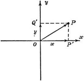
Fig. 12. Rectangular coördinates of a point.
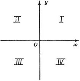
Fig. 13. The four quadrants.
The distance between the point P1 with coördinates x1, y1 and the point P2 with coördinates x2, y2 is given by the formula
(1) d2 = (x1 – x2)2 + (y1 – y2)2·
This follows immediately from the Pythagorean theorem, as may be seen from Figure 14.
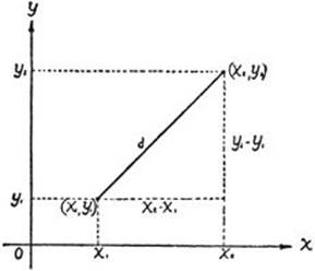
Fig. 14. The distance between two points.
*2. Equations of Lines and Curves
If C is a fixed point with coördinates x= a, y = b, then the locus of all points P having a given distance r from C is a circle with C as center and radius r. It follows from the distance formula (1) that the points of this circle have coördinates x, y which satisfy the equation
(2) (x – a)2 + (y – b)2 = r2·
This is called the equation of the circle, because it expresses the complete (necessary and sufficient) condition on the coördinates x, y of a point P
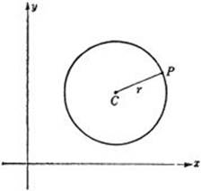
Fig. 15. The circle.
that lies on the circle around C with radius r. If the parentheses are expanded, equation (2) takes the form
(3) x2 + y2 – 2ax – 2by = k.
where k = r2 – a2 – b2. Conversely, if an equation of the form (3) is given, where a, b, and k are arbitrary constants such that k + a2 + b2 is positive, then by the algebraic process of “completing the square” we can write the equation in the form
(x – a)2 + (y – b)2 = r2,
where r2 = k + a2 + b2. It follows that the equation (3) defines a circle of radius r around the point C with coördinates a and b.
The equations of straight lines are even simpler in form. For example, the x-axis has the equation y = 0, since y = 0 for all points on the x-axis and for no other points. The y-axis has the equation x = 0. The lines through the origin bisecting the angles between the axes have the equations x= y and x = –y. It is easily shown that any straight line has an equation of the form
(4) ax + by = c,
where a, b, c are fixed constants characterizing the line. The meaning of equation (4) is again that all pairs of real numbers x, y which satisfy this equation are the coördinates of a point of the line, and conversely.
The reader may have learned that the equation
(5) ![]()
represents an ellipse (Fig. 16). This curve cuts the x-axis at the points A(p, 0) and A’(–p, 0), and the y-axis at B(0, q) and B’(0, –q). (The notation P(x, y) or simply (x, y) is used as a shorter way of writing “the point P with coördinates x and y.”) If p > q, the segment AA’, of length 2p, is called the major axis of the ellipse, while the segment BB’, of length 2q, is called the minor axis. This ellipse is the locus of all points P the sum of whose distances from the points ![]() and
and ![]() is 2p. As an exercise the reader may verify this by using formula (1). The points F and F’ are called the foci (singular, focus) of the ellipse, and the ratio
is 2p. As an exercise the reader may verify this by using formula (1). The points F and F’ are called the foci (singular, focus) of the ellipse, and the ratio ![]() is called the eccentricity of the ellipse.
is called the eccentricity of the ellipse.
An equation of the form
(6) ![]()
represents a hyperbola. This curve consists of two branches which cut the x-axis at A(p, 0) and A’(–p, 0) (Fig. 17) respectively. The segment A A’, of length 2p, is called the transverse axis of the hyperbola. The hyperbola approaches more and more nearly the two straight lines qx ± py = 0 as we go out farther and farther from the origin, but it never actually reaches these lines. They are called the asymptotes of the hyperbola. The hyperbola is the locus of all points P the difference of whose distances to the two points ![]() and
and ![]() is 2p. These points are again called the foci of the hyperbola; by its eccentricity we mean the ratio e =
is 2p. These points are again called the foci of the hyperbola; by its eccentricity we mean the ratio e = ![]() ·
·
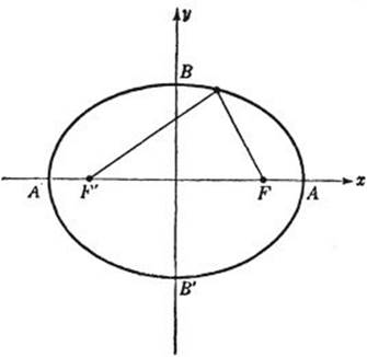
Fig. 16. The ellipse; F and F’ are the foci.
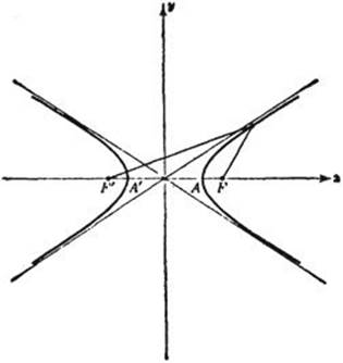
Fig. 17. The hyperbola; F and F’ are the foci.
The equation
(7) xy = 1
also defines a hyperbola, whose asymptotes now are the two axes (Fig. 18). The equation of this “equilateral” hyperbola indicates that the area of the rectangle determined by P is equal to 1 for every point P on the curve. An equilateral hyperbola whose equation is
(7a) xy = c,
c being a constant, is only a special case of the general hyperbola, just as the circle is a special case of the ellipse. The special character of the equilateral hyperbola lies in the fact that its two asymptotes (in this case the two coördinate axes) are perpendicular to each other.
For us the main point here is the fundamental idea that geometrical objects may be completely represented in numerical and algebraic terms, and that the same is true of geometrical operations. For example, if we want to find the point of intersection of two lines, we consider their two equations
ax + by = c
(8) a’x + b’y = c’.
The point common to the two lines is then found simply by determining its coördinates as the solution x, y of the two simultaneous equations (8). Similarly, the points of intersection of any two curves, such as the circle x2 + y2 – 2ax – 2by = k and the straight line ax + by = c, are found by solving the two corresponding equations simultaneously.
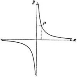
Fig. 18. The equilateral hyperbola xy = 1. The area xy of the rectangle determined by the point P (x, y) is equal to 1.