What Is Mathematics? An Elementary Approach to Ideas and Methods, 2nd Edition (1996)

§3. OTHER EXAMPLES OF TOPOLOGICAL THEOREMS

1. The Jordan Curve Theorem

A simple closed curve (one that does not intersect itself) is drawn in the plane. What property of this figure persists even if the plane is regarded as a sheet of rubber that can be deformed in any way? The length of the curve and the area that it encloses can be changed by a deformation. But there is a topological property of the configuration which is so simple that it may seem trivial: A simple closed curve C in the plane divides the plane into exactly two domains, an inside and an outside. By this is meant that the points of the plane fall into two classes—A, the outside of the curve, and B, the inside—such that any pair of points of the same class can be joined by a curve which does not cross C, while any curve joining a pair of points belonging to different classes must cross C. This statement is obviously true for a circle or an ellipse, but the self-evidence fades a little if one contemplates a complicated curve like the twisted polygon in Figure 128.

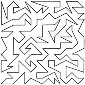
Fig. 128. Which points of the plane are inside this polygon?

This theorem was first stated by Camille Jordan (1838-1922) in his famous Cours d’Analyse, from which a whole generation of mathematicians learned the modern concept of rigor in analysis. Strangely enough, the proof given by Jordan was neither short nor simple, and the surprise was even greater when it turned out that Jordan’s proof was invalid and that considerable effort was necessary to fill the gaps in his reasoning. The first rigorous proofs of the theorem were quite complicated and hard to understand, even for many well-trained mathematicians. Only recently have comparatively simple proofs been found. One reason for the difficulty lies in the generality of the concept of “simple closed curve,” which is not restricted to the class of polygons or “smooth” curves, but includes all curves which are topological images of a circle. On the other hand, many concepts such as “inside,” “outside,” etc., which are so clear to the intuition, must be made precise before a rigorous proof is possible. It is of the highest theoretical importance to analyze such concepts in their fullest generality, and much of modern topology is devoted to this task. But one should never forget that in the great majority of cases that arise from the study of concrete geometrical phenomena it is quite beside the point to work with concepts whose extreme generality creates unnecessary difficulties. As a matter of fact, the Jordan curve theorem is quite simple to prove for the reasonably well-behaved curves, such as polygons or curves with continuously turning tangents, which occur in most important problems. We shall prove the theorem for polygons in the appendix to this chapter.

2. The Four Color Problem

From the example of the Jordan curve theorem one might suppose that topology is concerned with providing rigorous proofs for the sort of obvious assertions that no sane person would doubt. On the contrary, there are many topological questions, some of them quite simple in form, to which the intuition gives no satisfactory answer. An example of this kind is the renowned “four color problem.”

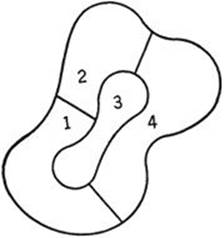
Fig. 129. Coloring a map.

In coloring a geographical map it is customary to give different colors to any two countries that have a portion of their boundary in common. It has been found empirically that any map, no matter how many countries it contains nor how they are situated, can be so colored by using onlyfour different colors. It is easy to see that no smaller number of colors will suffice for all cases. Figure 129 shows an island in the sea that certainly cannot be properly colored with less than four colors, since it contains four countries, each of which touches the other three.

The fact that no map has yet been found whose coloring requires more than four colors suggests the following mathematical theorem: For any subdivision of the plane into non-overlapping regions, it is always possible to mark the regions with one of the numbers 1, 2, 3, 4 in such a way that no two adjacent regions receive the same number. By “adjacent” regions we mean regions with a whole segment of boundary in common; two regions which meet at a single point only or at a finite number of points (such as the states of Colorado and Arizona) will not be called adjacent, since no confusion would arise if they were colored with the same color.

The problem of proving this theorem seems to have been first proposed by Moebius in 1840, later by DeMorgan in 1850, and again by Cayley in 1878. A “proof” was published by Kempe in 1879, but in 1890 Heawood found an error in Kempe’s reasoning. By a revision of Kempe’s proof, Heawood was able to show that five colors are always sufficient. (A proof of the five color theorem is given in the appendix to this chapter.) Despite the efforts of many famous mathematicians, the matter essentially rests with this more modest result: It has been proved that five colors suffice for all maps and it is conjectured that four will likewise suffice. But, as in the case of the famous Fermat theorem (see p. 42), neither a proof of this conjecture nor an example contradicting it has been produced, and it remains one of the great unsolved problems in mathematics. The four color theorem has indeed been proved for all maps containing less than thirty-eight regions. In view of this fact it appears that even if the general theorem is false it cannot be disproved by any very simple example.

In the four color problem the maps may be drawn either in the plane or on the surface of a sphere. The two cases are equivalent: any map on the sphere may be represented on the plane by boring a small hole through the interior of one of the regions A and deforming the resulting surface until it is flat, as in the proof of Euler’s theorem. The resulting map in the plane will be that of an “island” consisting of the remaining regions, surrounded by a “sea” consisting of the region A. Conversely, by a reversal of this process, any map in the plane may be represented on the sphere. We may therefore confine ourselves to maps on the sphere. Furthermore, since deformations of the regions and their boundary lines do not affect the problem, we may suppose that the boundary of each region is a simple closed polygon composed of circular arcs. Even thus “regularized,” the problem remains unsolved; the difficulties here, unlike those involved in the Jordan curve theorem, do not reside in the generality of the concepts of region and curve.

A remarkable fact connected with the four color problem is that for surfaces more complicated than the plane or the sphere the corresponding theorems have actually been proved, so that, paradoxically enough, the analysis of more complicated geometrical surfaces appears in this respect to be easier than that of the simplest cases. For example, on the surface of a torus (see Figure 123), whose shape is that of a doughnut or an inflated inner tube, it has been shown that any map may be colored by using seven colors, while maps may be constructed containing seven regions, each of which touches the other six.

*3. The Concept of Dimension

The concept of dimension presents no great difficulty so long as one deals only with simple geometric figures such as points, lines, triangles, and polyhedra. A single point or any finite set of points has dimension zero, a line segment is one-dimensional, and the surface of a triangle or of a sphere two-dimensional. The set of points in a solid cube is three-dimensional. But when one attempts to extend this concept to more general point sets, the need for a precise definition arises. What dimension should be assigned to the point set R consisting of all points on the x-axis whose coordinates are rational numbers? The set of rational points is dense on the line and might therefore be considered to be one-dimensional, like the line itself. On the other hand, there are irrational gaps between any pair of rational points, as between any two points of a finite point set, so that the dimension of the set R might also be considered to be zero.

An even more knotty problem arises if one tries to assign a dimension to the following curious point set, first considered by Cantor. From the unit segment remove the middle third, consisting of all points x such that 1/3 < x < 2/3. Call the remaining set of points C₁. Now from C₁ remove the middle third of each of its two segments, leaving a set which we call C₃. Repeat this process by removing the middle third of each of the four intervals of C₂, leaving a set C₂, and proceed in this manner to form sets C₄, C₅, C₆, · · ·. Denote by C the set of points on the unit segment that are left after all these intervals have been removed, i.e. C is the set of points common to the infinite sequence of sets C₁, C₂, · · ·. Since one interval, of length 1/3, was removed at the first step; two intervals, each of length 1/3², at the second step; etc.; the total length of the segments removed is

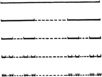
Fig. 130. Cantor’s point set.

The infinite series in parentheses is a geometrical series whose sum is 1/(1 – 2/3) = 3; hence the total length of the segments removed is 1. Still there remain points in the set C. Such, for example, are the points 1/3, 2/3, 1/9, 2/9, 7/9, 8/9, · · ·, by which the successive segments are trisected. As a matter of fact, it is easy to show that C will consist precisely of all those points x whose expansions in the form of infinite triadic fractions can be written in the form

where each a_i is either 0 or 2, while the triadic expansion of every point removed will have at least one of the numbers a_i, equal to 1.

What shall be the dimension of the set C? The diagonal process used to prove the non-denumerability of the set of all real numbers can be so modified as to yield the same result for the set C. It would seem, therefore, that the set C should be one-dimensional. Yet C contains no complete interval, no matter how small, so that C might also be thought of as zero-dimensional, like a finite set of points. In the same spirit, we might ask whether the set of points of the plane, obtained by erecting at each rational point or at each point of the Cantor set C a segment of unit length, should be considered to be one-dimensional or two-dimensional.

It was Poincaré who (in 1912) first called attention to the need for a deeper analysis and a precise definition of the concept of dimensionality. Poincaré observed that the line is one-dimensional because we may separate any two points on it by cutting it at a single point (which is of dimension 0), while the plane is two-dimensional because in order to separate a pair of points in the plane we must cut out a whole closed curve (of dimension 1). This suggests the inductive nature of dimensionality: a space is n-dimensional if any two points may be separated by removing an (n – 1)-dimensional subset, and if a lower-dimensional subset will not always suffice. An inductive definition of dimensionality is also contained implicitly in Euclid’s Elements, where a one-dimensional figure is something whose boundary consists of points, a two-dimensional figure one whose boundary consists of curves, and a three-dimensional figure one whose boundary consists of surfaces.

In recent years an extensive theory of dimension has been developed. One definition of dimension begins by making precise the concept “point set of dimension 0.” Any finite set of points has the property that each point of the set can be enclosed in a region of space which can be made as small as we please, and which contains no points of the set on its boundary. This property is now taken as the definition of 0-dimensionality. For convenience, we say that an empty set, containing no points at all, has dimension –1. Then a point set S is of dimension 0 if it is not of dimension –1 (i.e. if S contains at least one point), and if each point of S can be enclosed within an arbitrarily small region whose boundary intersects S in a set of dimension –1 (i.e. whose boundary contains no points of S). For example, the set of rational points on the line is of dimension 0, since each rational point can be made the center of an arbitrarily small interval with irrational endpoints. The Cantor set C is also seen to be of dimension 0, since, like the set of rational points, it is formed by removing a dense set of points from the line.

So far we have defined only the concepts of dimension –1 and dimension 0. The definition of dimension 1 suggests itself at once: a set S of points is of dimension 1 if it is not of dimension –1 or 0, and if each point of S can be enclosed within an arbitrarily small region whose boundary intersects S in a set of dimension 0. A line segment has this property, since the boundary of any interval is a pair of points, which is a set of dimension 0 according to the preceding definition. Moreover, by proceeding in the same manner, we can successively define the concepts of dimension 2, 3, 4, 5, · · ·, each resting on the previous definitions. Thus a set S will be of dimension n if it is not of any lower dimension, and if each point of S can be enclosed within an arbitrarily small region whose boundary intersects S in a set of dimension n – 1. For example, the plane is of dimension 2, since each point of the plane can be enclosed within an arbitrarily small circle, whose circumference is of dimension 1.† No point set in ordinary space can have dimension higher than 3, since each point of space can be made the center of an arbitrarily small sphere whose surface is of dimension 2. But in modern mathematics the word “space” is used to denote any system of objects for which a notion of “distance” or “neighborhood” is defined (see p. 316), and these abstract “spaces” may have dimensions higher than 3. A simple example is Cartesian n-space, whose “points” are ordered arrays of n real numbers:

P = (x₁, x₂, x₃ · · · x_n),

Q = (y₁, y₂, y₃ · · · y_n);

with the “distance” between the points P and Q defined as

This space may be shown to have dimension n. A space which does not have dimension n for any integer n is said to be of dimension infinity. Many examples of such spaces are known.

One of the most interesting facts of dimension theory is the following characteristic property of two-, three- or, in general, n-dimensional figures. Consider first the two-dimensional case. If any simple two-dimensional figure is subdivided into sufficiently small regions (each of which is regarded as including its boundary), then there will necessarily be points where three or more of these regions meet, no matter what the shapes of the regions. In addition, there will exist subdivisions of the figure in which each point belongs to at most three regions of the subdivision. Thus, if the two-dimensional figure is a square, as in Figure 131, then a point will belong to the three regions, 1, 2, and 3, while for this particular subdivision no point belongs to more than three regions. Similarly, in the three-dimensional case it may be proved that, if a volume is covered by sufficiently small volumes, there always exist points common to at least four of the latter, while for a properly chosen subdivision no more than four will have a point in common.

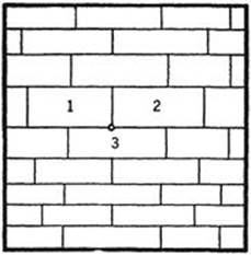
Fig. 131. The tiling theorem.

These observations suggest the following theorem, due to Lebesgue and Brouwer: If an n-dimensional figure is covered in any way by sufficiently small subregions, then there will exist points which belong to at least n + 1 of these subregions; moreover, it is always possible to find a covering by arbitrarily small regions for which no point will belong to more than n + 1 regions. Because of the method of covering considered here, this is known as the “tiling” theorem. It characterizes the dimension of any geometrical figure: those figures for which the theorem holds are n-dimensional, while all others are of some other dimension. For this reason it may be taken as the definition of dimensionality, as is done by some authors.

The dimension of any set is a topological feature of the set; no two figures of different dimensions can be topologically equivalent. This is the famous topological theorem of “invariance of dimensionality,” which gains in significance by comparison with the fact stated on page 85, that the set of points in a square has the same cardinal number as the set of points on a line segment. The correspondence there defined is not topological because the continuity conditions are violated.

*4. A Fixed Point Theorem

In the applications of topology to other branches of mathematics, “fixed point” theorems play an important rôle. A typical example is the following theorem of Brouwer. It is much less obvious to the intuition than most topological facts.

We consider a circular disk in the plane. By this we mean the region consisting of the interior of some circle, together with its circumference. Let us suppose that the points of this disk are subjected to any continuous transformation (which need not even be biunique) in which each point remains within the circle, although differently situated. For example, a thin rubber disk might be shrunk, turned, folded, stretched, or deformed in any way, so long as the final position of each point of the disk lies within its original circumference. Again, if the liquid in a glass is set into motion by stirring it in such a manner that particles on the surface remain on the surface but move around on it to other positions, then at any given instant the position of the particles on the surface defines a continuous transformation of the original distribution of the particles. The theorem of Brouwer now states: Each such transformation leaves at least one point fixed; that is, there exists at least one point whose position after the transformation is the same as its original position. (In the example of the surface of the liquid, the fixed point will in general change with the time, although for a simple circular rotation it is the center that is always fixed.) The proof of the existence of a fixed point is typical of the reasoning used to establish many topological theorems.

Consider the disk before and after the transformation, and assume, contrary to the statement of the theorem, that no point remains fixed, so that under the transformation each point moves to another point inside or on the circle. To each point P of the original disk attach a little arrow or “vector” pointing in the direction PP’, where P′ is the image of P under the transformation. At every point of the disk there is such an arrow, for every point was assumed to move somewhere else. Now consider the points on the boundary of the circle, with their associated vectors. All of these vectors point into the circle, since, by assumption, no points are transformed into points outside the circle. Let us begin at some point P₁ on the boundary and travel in the counterclockwise direction around the circle. As we do so, the direction of the vector will change, for the points on the boundary have variously pointed vectors associated with them. The directions of these vectors may be shown by drawing parallel arrows that issue from a single point in the plane. We notice that in traversing the circle once from P₁ around to P₁, the vector turns around and comes back to its original position. Let us call the number of complete revolutions made by this vector the “index” of the vectors on the circle; more precisely, we define the index as the algebraic sum of the various changes in angle of the vectors, so that each clockwise portion of a revolution is taken with a negative sign, while each counter-clockwise portion is regarded as positive. The index is the net result, which may a priori be any one of the numbers 0, ±1, ±2, ±3, · · ·, corresponding to a total change in angle of 0, ±360, ±720, · · · degrees. We now assert that the index equals 1; that is, the total change in the direction of the arrow amounts to exactly one positive revolution. To show this, we recall that the transformation vector at any point P on the circle is always directed inside the circle and never along the tangent. Now, if this transformation vector turns through a total angle different from the total angle through which the tangent vector turns (which is 360°, because the tangent vector obviously makes one complete positive revolution), then the difference between the total angles through which the tangent vector and the transformation vector turn will be some non-zero multiple of 360°, since each makes an integral number of revolutions. Hence the transformation vector must turn completely around the tangent at least once during the complete circuit from P₁ back to P₁, and since the tangent and the transformation vectors turn continuously, at some point of the circumference the transformation vector must point directly along the tangent. But this is impossible, as we have seen.

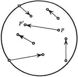
Fig. 132. Transformation vectors.

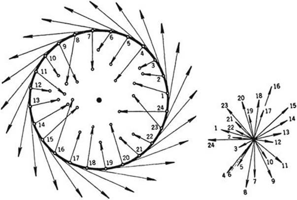
Fig. 133.

If we now consider any circle concentric with the circumference of the disk and contained within it, together with the corresponding transformation vectors on this circle, then the index of the transformation vectors on this circle must also be 1. For as we pass continuously from the circumference to any concentric circle, the index must change continuously, since the directions of the transformation vectors vary continuously from point to point within the disk. But the index can assume only integral values and therefore must be constantly equal to its original value 1, since a jump from 1 to some other integer would be a discontinuity in the behavior of the index. (The conclusion that a quantity that varies continuously but can assume only integral values is necessarily a constant is a typical bit of mathematical reasoning which intervenes in many proofs.) Thus we can find a concentric circle as small as we please for which the index of the corresponding transformation vectors is 1. But this is impossible, since by the assumed continuity of the transformation the vectors on a sufficiently small circle will all point in approximately the same direction as the vector at the center of the circle. Thus the total net change of their angles can be made as small as we please, less than 10°, say, by taking a small enough circle. Hence the index, which must be an integer, will be zero. This contradiction shows our initial hypothesis that there is no fixed point under the transformation to be untenable, and completes the proof.

The theorem just proved holds not only for a disk but also for a triangular or square region or any other surface that is the image of a disk under a topological transformation. For if A is any figure correlated with a disk by a biunique and continuous transformation, then a continuous transformation of A into itself which had no fixed point would define a continuous transformation of the disk into itself without a fixed point, which we have proved to be impossible. The theorem also holds in three dimensions for solid spheres or cubes, but the proof is not so simple.

Although the Brouwer fixed point theorem for the disk is not very obvious to the intuition, it is easy to show that it is an immediate consequence of the following fact, the truth of which is intuitively evident: It is impossible to transform continuously a circular disk into its circumference alone so that each point of the circumference remains fixed. We shall show that the existence of a fixed-point-free transformation of a disk into itself would contradict this fact. Suppose P → P′ were such a transformation; for each point P of the disk we could draw an arrow starting at P′ and continuing through P until it reached the circumference at some point P*. Then the transformation P → P* would be a continuous transformation of the whole disk into its circumference alone and would leave each point of the circumference fixed, contrary to the assumption that such a transformation is impossible. Similar reasoning may be used to establish the Brouwer theorem in three dimensions for the solid sphere or cube.

It is easy to see that some geometrical figures do admit continuous fixed-point-free transformations into themselves. For example, the ring-shaped region between two concentric circles admits as a continuous fixed-point-free transformation a rotation through any angle not a multiple of 360° about its center. The surface of a sphere admits the continuous fixed-point-free transformation that takes each point into its diametrically opposite point. But it may be proved, by reasoning analogous to that which we have used for the disk, that any continuous transformation which carries no point into its diametrically opposite point (e.g., any small deformation) has a fixed point.

Fixed point theorems such as these provide a powerful method for the proof of many mathematical “existence theorems” which at first sight may not seem to be of a geometrical character. A famous example is a fixed point theorem conjectured by Poincaré in 1912, shortly before his death. This theorem has as an immediate consequence the existence of an infinite number of periodic orbits in the restricted problem of three bodies. Poincaré was unable to confirm his conjecture, and it was a major achievement of American mathematics when in the following year G. D. Birkhoff succeeded in giving a proof. Since then topological methods have been applied with great success to the study of the qualitative behaviour of dynamical systems.

5. Knots

As a final example it may be pointed out that the study of knots presents difficult mathematical problems of a topological character. A knot is formed by first looping and interlacing a piece of string and then joining the ends together. The resulting closed curve represents a geometrical figure that remains essentially the same even if it is deformed by pulling or twisting without breaking the string. But how is it possible to give an intrinsic characterization that will distinguish a knotted closed curve in space from an unknotted curve such as the circle? The answer is by no means simple, and still less so is the complete mathematical analysis of the various kinds of knots and the differences between them. Even for the simplest case this has proved to be a sizable task. Consider the two trefoil knots shown in Figure 134. These two knots are completely symmetrical “mirror images” of one another, and are topologically equivalent, but they are not congruent. The problem arises whether it is possible to deform one of these knots into the other in a continuous way. The answer is in the negative, but the proof of this fact requires considerably more knowledge of the technique of topology and group theory than can be presented here.

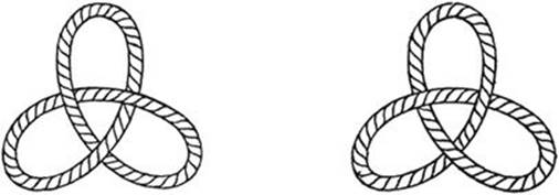
Fig. 134. Topologically equivalent knots that are not deformable into one another.