What Is Mathematics? An Elementary Approach to Ideas and Methods, 2nd Edition (1996)

§3. STATIONARY POINTS AND THE DIFFERENTIAL CALCULUS

1. Extrema and Stationary Points

In the preceding arguments the technique of the differential calculus was not used. As a matter of fact, our elementary methods are far more simple and direct than those of the calculus. As a rule in scientific thinking it is better to consider the individual features of a problem rather than to rely exclusively on general methods, although individual efforts should always be guided by a principle that clarifies the meaning of the special procedures used. This is indeed the rôle of the differential calculus in extremum problems. The modern search for generality represents only one side of the case, for the vitality of mathematics depends most decidedly on the individual color of problems and methods.

In its historic development, the differential calculus was strongly influenced by individual maximum and minimum problems. The connection between extrema and the differential calculus arises as follows. In Chapter VIII we shall make a detailed study of the derivative f′(x) of a functionf(x) and of its geometrical meaning. In brief, the derivative f′(x) is the slope of the tangent to the curve y = f(x) at the point (x, y). It is geometrically evident that at a maximum or minimum of a smooth curve y = f (x) the tangent to the curve must be horizontal, that is, its slope must be equal to zero. Thus we have the condition f′(x) = 0 for the extreme values of f(x).

To see what the vanishing of f′(x) means, let us examine the curve of Figure 191. There are five points, A, B, C, D, E, at which the tangent to this curve is horizontal; let the values of f(x) at these points be a, b, c, d, e respectively. The maximum of f(x) in the interval pictured is at D, the minimum at A. The point P also represents a maximum, in the sense that for all other points in the immediate neighborhood of B, f(x) is less than b, although f(x) is greater than b for points close to D. For this reason we call B a relative maximum of f(x), while D is the absolute maximum. Similarly, C represents a relative minimum and A the absolute minimum. Finally, at E, f(x) has neither a maximum nor a minimum, even though f′(x) = 0. From this it follows that the vanishing of f′(x) is a necessary, but not a sufficient condition for the occurrence of an extremum of a smooth function f(x); in other words, at any extremum, relative or absolute, f′(x)= 0, but not every point at which f′(x) = 0 need be an extremum. A point where the derivative vanishes, whether it is an extremum or not, is called a stationary point. By a more refined analysis, it is possible to arrive at more or less complicated conditions on the higher derivatives of f(x) which completely characterize the maxima, minima, and other stationary points.

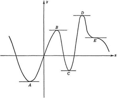
Fig. 191. Stationary points of a function.

2. Maxima and Minima of Functions of Several Variables. Saddle Points

There are problems of maxima and minima that cannot be expressed in terms of a function f(x) of one variable. The simplest such case is that of finding the extreme values of a function z = f(x, y) of two variables.

We can represent f(x, y) by the height z of a surface above the x, y-plane, which we may interpret, say, as a mountain landscape. A maximum of f(x, y) corresponds to a mountain top; a minimum, to the bottom of a depression or of a lake. In both cases, if the surface is smooth the tangent plane to the surface will be horizontal. But there are other points besides summits and the bottoms of valleys for which the tangent plane is horizontal; these are the points given by mountain passes. Let us examine these points in more detail. Consider as in Figure 192 two mountains A and Bon a range and two points C and D on different sides of the mountain range, and suppose that we wish to go from C to D. Let us first consider only the paths leading from C to D obtained by cutting the surface with some plane through C and D. Each such path will have a highest point. By changing the position of the plane, we change the path, and there will be one path CD for which the altitude of that highest point is least. The point E of maximum altitude on this path is a mountain pass, called in mathematical language a saddle point. It is clear that E is neither a maximum nor a minimum, since we can find points as near E as we please which are higher and lower than E. Instead of confining ourselves to paths that lie in a plane, we might just as well consider paths without this restriction. The characterization of the saddle point E remains the same.

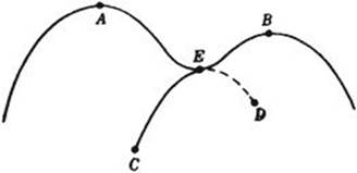
Fig. 192. A mountain pass.

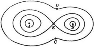
Fig. 193 The corresponding contour map.

Similarly, if we want to proceed from the peak A to the peak B, any particular path will have a lowest point; if again we consider only plane sections, there will be one path AB for which this lowest point is highest, and the minimum for this path is again at the point E found above. This saddle point E thus has the property of being a highest minimum or a lowest maximum; that is, a maxi-minimum or a mini-maximum. The tangent plane at E is horizontal; for, since E is the minimum point of AB, the tangent line to AB at E must be horizontal, and similarly, since E is the maximum point of CD, the tangent line to CD at E must be horizontal. The tangent plane, which is the plane determined by these lines, is therefore also horizontal. Thus we find three different types of points with horizontal tangent planes: maxima, minima, and saddle points; corresponding to these we have different types of stationary values of f(x, y).

Another way of representing a function f(x, y) is by drawing contour lines, such as those used in maps for representing altitudes (see p. 286). A contour line is a curve in the x, y-plane along which the function f(x, y) has a constant value; thus the contour lines are identical with the curves of the family f(x, y) = c. Through an ordinary point of the plane there passes exactly one contour line; a maximum or minimum is surrounded by closed contour lines; while at a saddle point several contour lines cross. In Figure 193 contour lines are drawn for the landscape of Figure 192, and the maximum-minimum property of E is evident: Any path connecting A and B and not going through E has to go through a region where f(x, y) < f(E), while the path AEB of Figure 192 has a minimum at E. In the same way we see that the value of f(x, y) at E is the smallest maximum for paths connecting C and D.

3. Minimax Points and Topology

There is an intimate connection between the general theory of stationary points and the concepts of topology. Here we can give only a brief indication of these ideas in connection with a simple example.

Let us consider the mountain landscape on a ring-shaped island B with the two boundaries C and C′. If again we represent the altitude above sea-level by u = f(x, y), with f(x, y) = 0 on C and C′ and f(x, y) > 0 in the interior of B, then there must exist at least one mountain pass on the island, shown in Figure 194 by the point where the contour lines cross. Intuitively, this can be seen if one tries to go from C to C′ in such a way that one’s path does not rise higher than necessary. Each path from C to C′ must possess a highest point, and if we select that path whose highest point is as low as possible, then the highest point of this path is a saddle point of u = f (x, y). (There is a trivial exception when a horizontal plane is tangent to the mountain crest all around the ring.) For a domain bounded by p curves there must exist, in general, at least p – 1 stationary points of minimax type. Similar relations have been discovered by Marston Morse to hold in higher dimensions, where there is a greater variety of topological possibilities and of types of stationary points. These relations form the basis of the modern theory of stationary points.

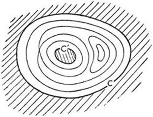
Fig. 194. Stationary points in a doubly connected region.

4. The Distance from a Point to a Surface

For the distance between a point P and a closed curve there are (at least) two stationary values, a minimum and a maximum. Nothing new occurs if we try to extend this result to three dimensions, so long as we consider a surface C topologically equivalent to a sphere, e.g. an ellipsoid. But new phenomena appear if the surface is of higher genus, e.g. a torus. There is still a shortest and a longest distance from P to a torus C, both segments being perpendicular to C. In addition we find extrema of different types representing maxima of minima or minima of maxima. To find them, we draw on the torus a closed “meridian” circle L, as in Figure 195, and we seek on L the point Q nearest to P. Then we try to move L so that the distance PQ becomes: a) a minimum. This Q is simply the point on C nearest to P. b) a maximum. This yields another stationary point. We could just as well seek on L the point farthest from P, and then find L such that this maximum distance is: c) a maximum, which will be attained at the point on C farthest from P. d) a minimum. Thus we obtain four different stationary values of the distance.

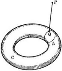
Fig. 195

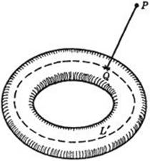
Fig. 196

* Exercise: Repeat the reasoning with the other type L′ of closed curve on C that cannot be contracted to a point, as in Figure 196.