What Is Mathematics? An Elementary Approach to Ideas and Methods, 2nd Edition (1996)

§6. EXTREMA AND INEQUALITIES

One of the characteristic features of higher mathematics is the important rôle played by inequalities. The solution of a maximum problem always leads, in principle, to an inequality which expresses the fact that the variable quantity under consideration is less than or at most equal to the maximum value provided by the solution. In many cases such inequalities have an independent interest. As an example we shall consider the important inequality between the arithmetical and geometrical means.

1. The Arithmetical and Geometrical Mean of Two Positive Quantities

We begin with a simple maximum problem which occurs very often in pure mathematics and its applications. In geometrical language it amounts to the following: Among all rectangles with a prescribed perimeter, to find the one with largest area. The solution, as one might expect, is the square. To prove this we reason as follows. Let 2a bt the prescribed perimeter of the rectangle. Then the fixed sum of the lengths x and y of two adjacent edges is x + y, while the variable are xy is to be made as large as possible. The “arithmetical mean” of and y is simply

We shall also introduce the quantity

so that

x = m + d, y = m – d,

and therefore

Since d² is greater than zero except when d = 0, we immediately obtain the inequality

where the equality sign holds only when d = 0 and x = y = m.

Since x + y is fixed, it follows that , and therefore the area xy, is a maximum when x = y. The expression

where the positive square root is meant, is called the “geometrical mean” of the positive quantities x and y; the inequality (1) expresses the fundamental relation between the arithmetical and geometrical means.

The inequality (1) also follows directly from the fact that the expression

is necessarily non-negative, being a square, and is zero only for x = y.

A geometrical derivation of the inequality may be given by considering the fixed straight line x + y = 2m in the plane, together with the family of curves xy = c, where c is constant for each of these curves (hyperbolas) and varies from curve to curve. As is evident from Figure 221, the curve with the greatest value of c having a point in common with the given straight line will be the hyperbola tangent to the line at the point x = y = m; for this hyperbola, therefore, c = m². Hence

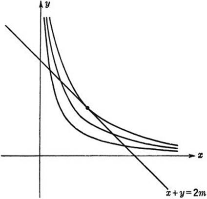
Fig. 221. Maximum xy for given x + y.

It should be remarked that any inequality, f(x, y) ≤ g(x, y), can be read both ways and therefore gives rise to a maximum as well as to a minimum property. For example, (1) also expresses the fact that among all rectangles of given area the square has the least perimeter.

2. Generalization to n Variables

The inequality (1) between the arithmetical and geometrical means of two positive quantities can be extended to any number n of positive quantities, denoted by x₁, x₂, · · ·, x_n. We call

their arithmetical mean, and

their geometrical mean, where the positive nth root is meant. The general theorem states that

and that g = m only if all the x_i are equal.

Many different and ingenious proofs of this general result have been devised. The simplest way is to reduce it to the same reasoning used in Article 1 by setting up the following maximum problem: To partition a given positive quantity C into n positive parts, C = x₁ + · · · + x_n, so that the product P = x₁x₂ · · · x₂ shall be as large as possible. We start with the assumption—apparently obvious, but analyzed later in §7—that a maximum for P exists and is attained by a set of values

x₁ = a₁, · · ·, x_n = a_n.

All we have to prove is that a₁ = a₂ = · · · = a_n, for in this case g = m. Suppose this is not true—for example, that a₁ ≠ a₂. We consider the n quantities

x₁ = s, x₂ = s, x₃ = a₃,· · ·, x_n = a_n,

where

In other words, we replace the quantities a_i, by another set in which only the first two are changed and made equal, while the total sum C is retained. We can write

a₁ = s + d, a₂ = s – d,

where

The new product is

P′ = s² · a₃ · · · a_n,

while the old product is

P= (s + d)·(s – d)·a₃ · · · a_n = (s² – d²)·a₃ · · · a_n,

so that obviously, unless d = 0,

P < P′,

contrary to the assumption that P was the maximum. Hence d = 0 and a₁ = a₂. In the same way we can prove that a₁ = a_i, where a_i is any one of the a’s; it follows that all the a’s are equal. Since g = m when all the x_i are equal, and since we have shown that only this gives the maximum value of g, it follows that g < m otherwise, as stated in the theorem.

3. The Method of Least Squares

The arithmetical mean of n numbers, x₁, · · ·, x_n, which need not be assumed all positive in this article, has an important minimum property. Let u be an unknown quantity that we want to determine as accurately as possible with some measuring instrument. To this end we make a numbern of readings which may yield slightly different results, x₁, · · ·, x_n, due to various sources of experimental error. Then the question arises, what value of u is to be accepted as most trustworthy? It is customary to select for this “true” or “optimal” value the arithmetical mean . To give a real justification for this assumption one must enter into a detailed discussion of the theory of probability. But we can at least point out a minimum property of m which makes it a reasonable choice. Let u be any possible value for the quantity measured. Then the differences u – x₁, · · ·, u – x_n are the deviations of this value from the different readings. These deviations can be partly positive, partly negative, and the tendency will naturally be to assume as the optimal value for u one for which the total deviation is in some sense as small as possible. Following Gauss, it is customary to take, not the deviations themselves, but their squares, (u – x_i)², as appropriate measures of inaccuracy, and to choose as the optimal value among all the possible values for u one such that the sum of the squares of the deviations

(u – x₁)² + (u – x₂)² + · · · + (u – x_n)²

is as small as possible. This optimal value for u is exactly the arithmetic mean m, and it is this fact that constitutes the point of departure in Gauss’s important “method of least squares.” We can prove the italicized statement in an elegant way. By writing

(u – x_i)= (m – x_i) + (u – m),

we obtain

(u – x_i)² = (m – x_i)² + (u – m)² + 2(m – x_i)(u – m).

Now add all these equations for i = 1, 2, · · ·, n. The last terms yield 2(u – m)(nm – x₁ – · · · – x_n), which is zero because of the definition of m; consequently we retain

(u – x₁)² + · · · + (u – x_n)² = (m – x₁)² + · · · + (m – x_n)² + n(m – u).²

This shows that

(u – x₁)² + · · · + (u – x_n)² ≥ (m – x₁)² + · · · + (m – x_n)²,

and that the equality sign holds only for u = m, which is exactly what we were to prove.

The general method of least squares takes this result as a guiding principle in more complicated cases when the problem is to decide on a plausible result from slightly incompatible measurements. For example, suppose we have measured the coördinates of n points x_i, y_i of a theoretically straight line, and suppose that these measured points do not lie exactly on a straight line. How shall we draw the line that best fits the n observed points? Our previous result suggests the following procedure, which, it is true, might be replaced by equally reasonable variants. Let y = ax + brepresent the equation of the line, so that the problem is to find the coefficients a and b. The distance in the y direction from the line to the point x_i, y_i is given by y_i – (ax_i + b) = y_i, – ax_i, – b, with a positive or negative sign according as the point is above or below the line. Hence the square of this distance is (y_i, – ax_i – b)², and the method is simply to determine α and b in such a way that the expression

(y₁ – ax₁ – b)² + · · · + (y_n – ax_n – b)²

attains its least possible value. Here we have a minimum problem involving two unknown quantities, a and b. The detailed discussion of the solution, though quite simple, is omitted here.