What Is Mathematics? An Elementary Approach to Ideas and Methods, 2nd Edition (1996)

§10. THE CALCULUS OF VARIATIONS

1. Introduction

The isoperimetric problem is one example, probably the oldest, of a large class of important problems to which attention was called in 1696 by Johann Bernoulli. In Acta Eruditorum, the great scientific journal of the time, he posed the following “brachistochrone” problem: Imagine a particle constrained to slide without friction along a certain curve joining a point A to a lower point B. If the particle is allowed to fall under the influence of gravity alone, along which such curve will the time required for the descent be least? It is easy to see that the falling particle will require different lengths of time for different paths. The straight line by no means affords the quickest journey, nor is the circular arc or any other elementary curve the answer. Bernoulli boasted of having a wonderful solution which he would not immediately publish in order to incite the greatest mathematicians of the time to try their skill at this new type of mathematical question. In particular, he challenged his elder brother Jacob, with whom he was at the time engaged in a bitter feud, and whom he publicly described as incompetent, to solve the problem. Mathematicians immediately recognized the different character of the brachistochrone problem. While heretofore, in problems treated by the differential calculus, the quantity to be minimized depended only on one or more numerical variables, in this problem the quantity under consideration, the time of descent, depends on the whole curve, and this makes for an essential difference, taking the problem out of the reach of the differential calculus or any other method known at the time.

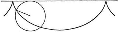
Fig. 236. Tho cycloid.

The novelty of the problem—apparently the isoperimetric property of the circle was not clearly recognized as of the same nature—fascinated the contemporary mathematicians all the more when the solution turned out to be the cycloid, a curve that had just been discovered. (We recall the definition of the cycloid: it is the locus of a point on the circumference of a circle that rolls without slipping along a straight line, as shown in Fig. 236.) This curve had been brought into connection with interesting mechanical problems, especially with the construction of an ideal pendulum. Huygens had discovered that an ideal mass point which oscillates without friction under the influence of gravity on a vertical cycloid has a period of oscillation independent of the amplitude of the motion. On a circular path, such as is provided by an ordinary pendulum, this independence is only approximately true, and this was considered a drawback to the use of pendulums for precision clocks. The cycloid was honored by the name of tautochrone; now it acquired the new title of brachistochrone.

2. The Calculus of Variations. Fermat’s Principle in Optics

Of the different ways in which the solution to the brachistochrone problem was found by the Bernoullis and others we shall presently explain one of the most original. The first methods were of a more or less special character, adapted to the specific problem. But it did not take long before Euler and Lagrange (1736–1813) evolved more general methods for solving extremum problems in which the independent element was not a single numerical variable or a finite number of such variables, but a whole curve or function or even a system of functions. The new method for solving such problems was called the calculus of variations.

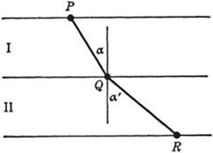
Fig. 237. Refraction of a light ray.

It is not possible to describe here the technical aspects of this branch of mathematics or to go deeper into the discussion of specific problems. The calculus of variations has many applications in physics. It was observed long ago that natural phenomena often follow some pattern of maxima and minima. As we have seen, Heron of Alexandria recognized that the reflection of a light ray in a plane mirror can be described by a minimum principle. Fermat, in the seventeenth century, took the next step: he observed that the law of refraction of light can also be stated in terms of a minimum principle. It is well known that the path of light travelling from one homogeneous medium into another is bent at the boundary. Thus in Figure 237, a light ray going from P in the upper medium where the velocity is υ to R in the lower medium where the velocity is w will follow a path PQR. The empirical law found by Snell (1591–1626) states that the path consists of two straight segments, PQ and QR, forming angles α, α′ with the normal determined by the conditions sin α/sin α′ = υ/w. By means of the calculus Fermat proved that this path is such that the time taken for the light ray to go from P to R is a minimum, i.e. smaller than it would be along any other connecting path. Thus Heron’s law of reflection was supplemented sixteen hundred years later by a similar and equally important law of refraction.

Fermat generalized the statement of this law so as to include curved surfaces of discontinuity between media, such as the spherical surfaces used in lenses. In this case the statement still holds that light follows a path along which the time taken is a minimum relative to the time that would be required for the light to describe any other possible path between the same two points. Finally, Fermat considered any optical system in which the velocity of light varies in a prescribed way from point to point, as it does in the atmosphere. He divided the continuous inhomogeneous medium into thin slabs, in each of which the velocity of light is approximately constant, and imagined this medium replaced by another in which the velocity is actually constant in each slab. Then he could again apply his principle, going from each slab to the next. By letting the thickness of the slabs tend to zero, he arrived at the general Fermat principle of geometrical optics: In an inhomogeneous medium, a light ray travelling between two points follows a path along which the time taken is a minimum with respect to all paths joining the two points. This principle has been of the utmost importance, not only theoretically, but in practical geometrical optics. The technique of the calculus of variations applied to this principle provides the basis for calculating lens systems.

Minimum principles have also become dominant in other branches of physics. It was observed that stable equilibrium of a mechanical system is attained if the system is arranged in such a way that its “potential energy” is a minimum. As an example, let us consider a flexible homogeneous chain suspended at its two ends and allowing full play to the force of gravity. The chain will then assume a form in which its potential energy is a minimum. In this case the potential energy is determined by the height of the center of gravity above some fixed axis. The curve in which the chain hangs is called a catenary, and resembles superficially a parabola.

Not only the laws of equilibrium, but also those of motion, are dominated by maximum and minimum principles. It was Euler who obtained the first clear ideas about these principles, while philosophically and mystically inclined speculators, such as Maupertuis (1698–1759), were not able to separate the mathematical statements from hazy ideas about “God’s intention to regulate physical phenomena by a general principle of highest perfection.” Euler’s variational principles of physics, rediscovered and extended by the Irish mathematician W. R. Hamilton (1805–1865), have proved to be among the most powerful tools in mechanics, optics, and electrodynamics, with many applications to engineering. Recent developments in physics—relativity and quantum theory—are full of examples revealing the power of the calculus of variations.

3. Bernoulli’s Treatment of the Brachistochrone Problem

The early method developed for the brachistochrone problem by Jacob Bernoulli can be understood with comparatively little technical knowledge. We start with the fact, taken from mechanics, that a mass point falling from rest at A along any curve C will have at any point P a velocity proportional to , where h is the vertical distance from A to P; that is, , where c is a constant. Now we replace the given problem by a slightly different one. We dissect the space into many thin horizontal slabs, each of thickness d, and assume for the moment that the velocity of the moving particle changes, not continuously, but in little jumps from slab to slab, so that in the first slab adjacent to A the velocity is , in the second , and in the nth slab , where h is the vertical distance from A to P (see Fig. 238). If this problem is considered, then there are really only a finite number of variables. In each slab the path must be a straight segment, no existence problem arises, the solution must be a polygon, and the only question is how to determine its corners. According to the minimum principle for the law of simple refraction, in each pair of successive slabs the motion from P to R by way of Q must be such that, with P and R fixed, Q provides the shortest possible time. Hence the following “refraction law” must hold:

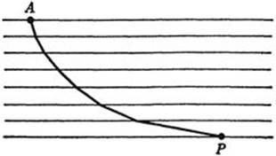
Fig. 238.

Repeated application of this reasoning yields the succession of equalities

(1) 

where α_n is the angle between the polygon in the nth slab and the vertical.

Now Bernoulli imagines the thickness d to become smaller and smaller, tending to zero, so that the polygon just obtained as the solution of the approximate problem tends to the desired solution of the original problem. In this passage to the limit the equalities (1) are not affected, and therefore Bernoulli concludes that the solution must be a curve C with the following property: If α is the angle between the tangent and the vertical at any point P of C, and h is the vertical distance of P from the horizontal line through A, then is constant for all points P of C. It can be shown very simply that this property characterizes the cycloid.

Bernoulli’s “proof” is a typical example of ingenious and valuable mathematical reasoning which, at the same time, is not at all rigorous. There are several tacit assumptions in the argument, and their justification would be more complicated and lengthy than the argument itself. For example, the existence of a solution C, and the fact that the solution of the approximate problem approximates the actual solution, were both assumed. The question as to the intrinsic value of heuristic considerations of this type certainly deserves discussion, but would lead us too far astray.

4. Geodesics on a Sphere. Geodesics and Maxi-Minima

In the introduction to this chapter we mentioned the problem of finding the shortest arcs joining two given points of a surface. On a sphere, as is shown in elementary geometry, these “geodesics” are arcs of great circles. Let P and Q be two (not diametrically opposite) points on a sphere, and c the shorter connecting arc of the great circle through P and Q. Then the question presents itself, what is the longer arc c′ of the same great circle? Certainly it does not give the minimum length, nor can it give the maximum length for curves joining P and Q, since arbitrarily long curves between P and Q can be drawn. The answer is that c′ solves a maxi-minimum problem. Consider a point S on a fixed great circle separating P and Q; we ask for the shortest connection between P and Q on the sphere passing through S. Of course, the minimum is given by a curve consisting of two small arcs of great circles PS and QS. Now we seek a position of the point S for which this smallest distance PSQ becomes as large as possible. The solution is: S must be such that PSQ is the longer arc c′ of the great circle PQ. We may modify the problem by first seeking the path of shortest length from P to Q passing through n prescribed points, S₁, S₂,..., S_n, on the sphere, and then seeking to determine the points S₁,..., S_n so that this minimum length becomes as large as possible. The solution is given by a path on the great circle joining P and Q, but this path winds around the sphere so often that it passes through the points diametrically opposite P and Q exactly n times.

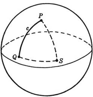
Fig. 239. Geodesics on a sphere

This example of a maximum-minimum problem is typical of a wide class of questions in the calculus of variations that have been studied with great success by methods developed by Morse and others.