What Is Mathematics? An Elementary Approach to Ideas and Methods, 2nd Edition (1996)
CHAPTER VIII. THE CALCULUS
INTRODUCTION
With an absurd oversimplification, the “invention” of the calculus is sometimes ascribed to two men, Newton and Leibniz. In reality, the calculus is the product of a long evolution that was neither initiated nor terminated by Newton and Leibniz, but in which both played a decisive part. Scattered over seventeenth century Europe, for the most part outside the schools, was a group of spirited scientists who strove to continue the mathematical work of Galileo and Kepler. By correspondence and travel these men maintained close contact. Two central problems held their attention. First, the problem of tangents: to determine the tangent lines to a given curve, the fundamental problem of the differential calculus. Second, the problem of quadrature: to determine the area within a given curve, the fundamental problem of the integral calculus. Newton’s and Leibniz’ great merit is to have clearly recognized the intimate connection between these two problems. In their hands the new unified methods became powerful instruments of science. Much of the success was due to the marvelous symbolic notation invented by Leibniz. His achievement is in no way diminished by the fact that it was linked with hazy and untenable ideas which are apt to perpetuate a lack of precise understanding in minds that prefer mysticism to clarity. Newton, by far the greater scientist, appears to have been mainly inspired by Barrow (1630-1677), his teacher and predecessor at Cambridge. Leibniz was more of an outsider. A brilliant lawyer, diplomat, and philosopher, one of the most active and versatile minds of his century, he learned the new mathematics in an incredibly short time from the physicist Huygens while visiting Paris on a diplomatic mission. Soon afterwards he published results that contain the nucleus of the modern calculus. Newton, whose discoveries had been made much earlier, was averse to publication. Moreover, although he had originally found many of the results in his masterpiece, the Principia, by the methods of the calculus, he preferred a presentation in the style of classical geometry, and almost no trace of the calculus appears explicitly in the Principia. Only later were his papers on the method of “fluxions” published. Soon his admirers started a bitter feud over priority with the friends of Leibniz. They accused the latter of plagiarism, although in an atmosphere saturated with the elements of a new theory, nothing is more natural than simultaneous and independent discovery. The resulting quarrel over priority in the “invention” of the calculus set an unfortunate example for the overemphasis on questions of precedence and claims to intellectual property that is apt to poison the atmosphere of natural scientific contact.
In the mathematical analysis of the seventeenth and most of the eighteenth centuries, the Greek ideal of clear and rigorous reasoning seemed to have been discarded. “Intuition” and “instinct” replaced reason in many important instances. This only encouraged an uncritical belief in the superhuman power of the new methods. It was generally thought that a clear presentation of the results of the calculus was not only unnecessary but impossible. Had not the new science been in the hands of a small group of extremely competent men, serious errors and even debacle might have resulted. These pioneers were guided by a strong instinctive feeling that kept them from going far astray. But when the French Revolution opened the way to an immense extension of higher learning, when increasingly large numbers of men wished to participate in scientific activity, the critical revision of the new analysis could no longer be postponed. This challenge was successfully met in the nineteenth century, and today the calculus can be taught without a trace of mystery and with complete rigor. There is no longer any reason why this basic instrument of the sciences should not be understood by every educated person.
This chapter is intended to serve as an elementary introduction in which the emphasis is on understanding the basic concepts rather than on formal manipulation. Intuitive language will be used throughout, but always in a manner consistent with precise concepts and clear procedure.
§1. THE INTEGRAL
1. Area as a Limit
In order to calculate the area of a plane figure we choose as the unit of area a square whose sides are of unit length. If the unit of length is the inch, the corresponding unit of area will be the square inch; i.e. the square whose sides are of length one inch. On the basis of this definition it is very easy to calculate the area of a rectangle. If p and q are the lengths of two adjacent sides measured in terms of the unit of length, then the area of the rectangle is pq square units, or, briefly, the area is equal to the product pq. This is true for arbitrary p and q, rational or not. For rational pand q we obtain this result by writing p = m/n, q = m′/n′, with integers m, n, m′, n′. Then we find the common measure 1/N = 1/nn′ of the two edges, so that p = mn′·1/N, q = nm′ · 1/N. Finally, we subdivide the rectangle into small squares of side 1/N and area 1/N2. The number of such squares is nm′·mn′ and the total area is nm′mn′ · 1/N2 = nm′mn′/n2 n′2 = m/n · m′/n′ = pq. If p and q are irrational, the same result is obtained by first replacing p and q by approximate rational numbers pr and qr respectively, and then letting pr and qr tend to p and q.
It is geometrically obvious that the area of a triangle is equal to half the area of a rectangle with the same base b and altitude h; hence the area of a triangle is given by the familiar expression ½bh. Any domain in the plane bounded by one or more polygonal lines can be decomposed into triangles; its area, therefore, can be obtained as the sum of the areas of these triangles.
The need for a more general method of computing areas arises when we ask for the area of a figure bounded, not by polygons, but by curves. How shall we determine, for example, the area of a circular disk or of a segment of a parabola? This crucial question, which is at the base of the integral calculus, was treated as early as the third century B.C. by Arch medes, who calculated such areas by a process of “exhaustion.” With Archimedes and the great mathematicians until the time of Gauss, we may take the “naive” attitude that curvilinear areas are intuitively given entities, and that the question is not to define, but to compute them (see, however, the discussion on p. 464). We inscribe in the domain an approximating domain with a polygonal boundary and a well defined area. By choosing another polygonal domain which includes the former we obtain a better approximation to the given domain. Proceeding in this way, we can gradually “exhaust” the whole area, and we obtain the area of the given domain as the limit of the areas of a properly chosen sequence of inscribed polygonal domains with an increasing number of sides. The area of a circle of radius 1 may be computed in this way; its numerical value is denoted by the symbol π.
Archimedes carried out this general scheme for the circle and for the parabolic segment. During the seventeenth century many more cases were successfully treated. In each case, the actual calculation of the limit was made to depend on an ingenious device specially suited to the particular problem. One of the main achievements of the calculus was to replace these special and restricted procedures for the calculation of areas by a general and powerful method.
2. The Integral
The first basic concept of the calculus is that of integral. In this article we shall understand the integral as an expression of the area under a curve by means of a limit. If a positive continuous function y = f(x) is given, e.g. y = x2 or y = 1 + cos x, then we consider the domain bounded below by the segment on the x-axis from a coördinate a to a greater coördinate b, on the sides by the perpendiculars to the x-axis at these points, and above by the curve y = f(x). Our aim is to calculate the area A of this domain.
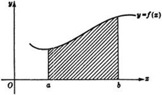
Fig. 259. The integral as an area.
Since such a domain cannot, in general, be decomposed into rectangles or triangles, no immediate expression of this area A is available for explicit calculation. But we can find an approximate value for A, and thus represent A as a limit, in the following way: We subdivide the interval from x = a to x = b into a number of small subintervals, erect perpendiculars at each point of subdivision, and replace each strip of the domain under the curve by a rectangle whose height is chosen somewhere between the greatest and the least height of the curve in that strip. The sum S of the areas of these rectangles gives an approximate value for the actual area A under the curve. The accuracy of this approximation will be better the larger the number of rectangles and the smaller the width of each individual rectangle. Thus we can characterize the exact area as a limit: If we form a sequence,
(1) S1, S2, S3, · · ·,
of rectangular approximations to the area under the curve in such a manner that the width of the widest rectangle in Sn tends to 0 as n increases, then the sequence (1) approaches the limit A,
(2) Sn → A,
and this limit A, the area under the curve, is independent of the particular way in which the sequence (1) is chosen, so long as the widths of the approximating rectangles tend to zero. (For example, Sn can arise from Sn-1 by adding one or more new points of subdivision to those defining Sn-1or the choice of points of subdivision for Sn can be entirely independent of the choice for Sn-1 ·) The area A of the domain, expressed by this limiting process, we call by definition the integral of the function f(x) from a to b. With a special symbol, the “integral sign,” it is written
(3) ![]()
The symbol ∫, the “dx,” and the name “integral” were introduced by Leibniz in order to suggest the way in which the limit is obtained. To explain this notation we shall repeat in more detail the process of approximation to the area A. At the same time the analytic formulation of the limiting process will make it possible to discard the restrictive assumptions f(x) ≥ 0 and b > a, and finally to eliminate the prior intuitive concept of area as the basis of our definition of integral (the latter will be done in the supplement, §1).
Let us subdivide the interval from a to b into n small subintervals, which, for simplicity only, we shall assume to be of equal width, (b — a)/n. We denote the points of subdivision by
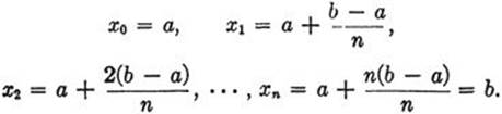
We introduce for the quantity (b — a)/n, the difference between consecutive x-values, the notation Δx (read, “delta x”),
![]()
where the symbol Δ means simply “difference” (it is an “operator” symbol, and must not be mistaken for a number.) We may choose as the height of each approximating rectangle the value of y = f(x) at the right-hand endpoint of the subinterval. Then the sum of the areas of these rectangles will be
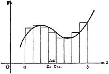
Fig. 260. Area approximated by small rectangles.
(4) Sn = f(x1) · Δ x + f(x2) · Δx + · · · + f(xn) · Δx,
which is abbreviated as
(5) ![]()
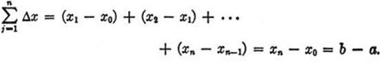
Here the symbol ![]() (read “sigma from j= 1 to n”) means the sum of all the expressions obtained by letting j assume in turn the values 1, 2, 3, · · ·, n.
(read “sigma from j= 1 to n”) means the sum of all the expressions obtained by letting j assume in turn the values 1, 2, 3, · · ·, n.
The use of the symbol Σ to express in concise form the result of a summation may be illustrated by the following examples:

Now we form a sequence of such approximations Sn in which n in creases indefinitely, so that the number of terms in each sum (5) increases, while each single term f(xi)Δx approaches 0 because of the factor Δ x = (b – a)/n. As n increases, this sum tends to the area A,
(6) ![]()
Leibniz symbolized this passage to the limit from the approximating sum Sn to A by replacing the summation sign ![]() by ∫ and the difference symbol Δ by the symbol d. (The summation symbol
by ∫ and the difference symbol Δ by the symbol d. (The summation symbol ![]() was usually written S in Leibniz’ time, and the symbol ∫ is merely a stylized S.) While Leibniz’ symbolism is very suggestive of the manner in which the integral is obtained as the limit of a finite sum, one must be careful not to attach too much significance to what is, after all, a pure convention as to how the limit shall be denoted. In the early days of the calculus, when the concept of limit was not clearly understood and certainly not always kept in mind, one explained the meaning of the integral by saying that “the finite difference Δx is replaced by the infinitely small quantity dx, and the integral itself is the sum of infinitely many infinitely small quantities f(x)dx.” Although the infinitely small has a certain attraction for speculative souls, it has no place in modern mathematics. No useful purpose is served by surrounding the clear notion of the integral with a fog of meaningless phrases. But even Leibniz was sometimes carried away by the suggestive power of his symbols; they work as if they denote a sum of “infinitely small” quantities with which one can nevertheless operate to a certain extent as with ordinary quantities. In fact, the word integral was coined to indicate that the whole or integral area A is composed of the “infinitesimal” parts f(x) dx. At any rate, it was almost a hundred years after Newton and Leibniz before it was clearly recognized that the limit concept and nothing else is the true basis for the definition of the integral. By firmly staying on this basis we may avoid all the haze, all the difficulties, and all the nonsense so disturbing in the early development of the calculus.
was usually written S in Leibniz’ time, and the symbol ∫ is merely a stylized S.) While Leibniz’ symbolism is very suggestive of the manner in which the integral is obtained as the limit of a finite sum, one must be careful not to attach too much significance to what is, after all, a pure convention as to how the limit shall be denoted. In the early days of the calculus, when the concept of limit was not clearly understood and certainly not always kept in mind, one explained the meaning of the integral by saying that “the finite difference Δx is replaced by the infinitely small quantity dx, and the integral itself is the sum of infinitely many infinitely small quantities f(x)dx.” Although the infinitely small has a certain attraction for speculative souls, it has no place in modern mathematics. No useful purpose is served by surrounding the clear notion of the integral with a fog of meaningless phrases. But even Leibniz was sometimes carried away by the suggestive power of his symbols; they work as if they denote a sum of “infinitely small” quantities with which one can nevertheless operate to a certain extent as with ordinary quantities. In fact, the word integral was coined to indicate that the whole or integral area A is composed of the “infinitesimal” parts f(x) dx. At any rate, it was almost a hundred years after Newton and Leibniz before it was clearly recognized that the limit concept and nothing else is the true basis for the definition of the integral. By firmly staying on this basis we may avoid all the haze, all the difficulties, and all the nonsense so disturbing in the early development of the calculus.
3. General Remarks on the Integral Concept. General Definition
In our geometrical definition of the integral as an area we assumed explicitly that f(x) is never negative throughout the interval [a, b] of integration, i.e. that no portion of the graph lies below the x-axis. But in our analytic definition of the integral as the limit of a sequence of sums Sn this assumption is superfluous. We simply take the small quantities f(xi) · Δx, form their sum, and pass to the limit; this procedure remains perfectly meaningful if some or all of the values f(xi) are negative. Interpreting this geometrically by means of areas (Fig. 261), we find the integral of f(x) to be the algebraic sum of the areas bounded by the graph and the x-axis, where areas lying below the x-axis are counted as negative and the others positive.
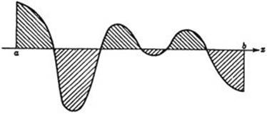
Fig. 261. Positive and negative areas.
It may happen that in applications we are led to integrals ![]() where b is less than a, so that (b – a)/n = Δx is a negative number. In our analytic definition we have f(xi) · Δx negative if f(xi) is positive and Δx negative, etc. In other words, the value of the integral will be the negative of the value of the integral from b to a. Thus we have the simple rule
where b is less than a, so that (b – a)/n = Δx is a negative number. In our analytic definition we have f(xi) · Δx negative if f(xi) is positive and Δx negative, etc. In other words, the value of the integral will be the negative of the value of the integral from b to a. Thus we have the simple rule
![]()
We must emphasize that the value of the integral remains the same even if we do not restrict ourselves to equidistant points xi of subdivision, or, what is the same, to equal x-differences Δx = xi+1 – xi ·. We may choose the xi in other ways, so that the differences Δxi+ = xi+1 – xi are not equal (and must accordingly be distinguished by subscripts). Even then the sums
Sn = f(x1)Δx0 + f(x2)Δx1 + · · · f(xn)Δxn-1
and also the sums
![]()
will tend to the same limit, the value of the integral ![]() , if only care is taken that with increasing n all the differences Δxi = xi+1 – xi tend to zero in such a way that the largest such difference for a given value of n approaches zero as n increases.
, if only care is taken that with increasing n all the differences Δxi = xi+1 – xi tend to zero in such a way that the largest such difference for a given value of n approaches zero as n increases.
Accordingly, the final definition of the integral is given by
(6a) ![]()
as n → ∞. In this limit vi may denote any point of the interval xi ≤ vi ≤ xi+1, and the only restriction for the subdivision is that the longest interval Δxi = xi+1 xi must tend to zero as n increases.
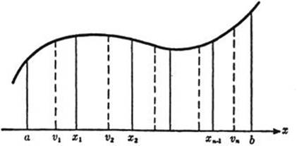
Fig. 262. Arbitrary subdivision in the general definition of integral.
The existence of the limit (6a) does not need a proof if we take for granted the concept of the area under a curve and the possibility of approximating this area by sums of rectangles. However, as will appear in a later discussion (p. 464), a closer analysis shows that it is desirable and even necessary for a logically complete presentation of the notion of integral to prove the existence of the limit for any continuous function f(x) without reference to a prior geometrical concept of area.
4. Examples of Integration. Integration of xr
Until now our discussion of the integral has been merely theoretical. The crucial question is whether the general pattern of forming a sum Sn and then passing to the limit actually leads to tangible results in concrete cases. Of course, this will require some additional reasoning adapted to the specific function f(x) for which the integral is to be found. When Archimedes two thousand years ago found the area of the parabolic segment, he performed what we now call the integration of the function f(x) = x2 by a very ingenious device; in the seventeenth century the forerunners of the modern calculus succeeded in solving problems of integration for simple functions such as xn, again by special devices. Only after much experience with specific cases was a general approach to the problem of integration found in the systematic methods of the calculus, and thus the scope of solvable individual problems was greatly widened. In the present article we shall discuss a few of the instructive special problems belonging to the “pre-calculus” stage, for nothing can better illustrate integration as a limiting process.
a) We start with a quite trivial example. If y = f(x) is a constant, for example f(x) = 2, then obviously the integral ![]() , understood as an area, is 2(b – a), since the area of a rectangle is equal to base times altitude. We shall compare this result with the definition of the integral (6) as a limit: If we substitute in (5) f(xi) = 2 for all values of j, we find that
, understood as an area, is 2(b – a), since the area of a rectangle is equal to base times altitude. We shall compare this result with the definition of the integral (6) as a limit: If we substitute in (5) f(xi) = 2 for all values of j, we find that
![]()
for every n, since
b) Almost as simple is the integration of f(x) = x. Here ![]() is the area of a trapezoid (Fig. 263), and this, by elementary geometry, is
is the area of a trapezoid (Fig. 263), and this, by elementary geometry, is
![]()
This result again agrees with the definition (6) of the integral, as is seen by an actual passage to the limit without making use of the geometrical figure: If we substitute f(x) = x in (5), then the sum Sn becomes
Using the formula (1) on page 12· for the arithmetical series 1 + 2 + 3 +... + n, we have
![]()
![]() , this is equal to
, this is equal to
![]()
If now we let n tend to infinity, the last term tends to zero, and we obtain
![]()
in conformity with the geometrical interpretation of the integral as an area.
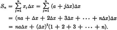
c) Less trivial is the integration of the function f(x) = x2. Archimedes used geometrical methods to solve the equivalent problem of finding the area of a segment of the parabola y = x2. We shall proceed analytically on the basis of the definition (6a). To simplify the formal calculation we choose 0 as the “lower limit” a of the integral; then
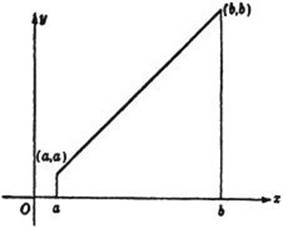
Fig. 263. Area of a trapezoid.
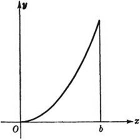
Fig. 264. Area under a parabola.
Δx = b/n. Since xi = j · Δx and f(xi) = j2(Δx)2, we obtain for Sn the expression
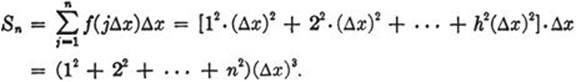
Now we can actually calculate the limit. Using the formula
![]()
established on page 14, and making the substitution Δx = b/n, we obtain
![]()
This preliminary transformation makes the passage to the limit an easy matter, since 1/n tends to zero as n increases indefinitely. Thus we obtain as limit simply ![]() , and thereby the result
, and thereby the result
![]()
Applying this result to the area from 0 to a we have
![]()
and by subtraction of the areas,
![]()
Exercise: Prove in the same way, using formula (5) on page 15 that
![]()
By developing general formulas for the sum 1k + 2k + · · · + nk of the kth powers of the integers from 1 to n, one can obtain the result
(7) ![]()
* Instead of proceeding in this way, we can obtain more simply an even more general result by utilizing our previous remark that we may calculate the integral by means of non-equidistant points of subdivision. We shall establish formula (7) not only for any positive integer k but for an arbitrary positive or negative rational number
k = u/v,
where u is a positive integer and v is a positive or negative integer. Only the value k = —1, for which formula (7) becomes meaningless, is excluded. We shall also suppose that 0 < a < b.
To obtain the integral formula (7), we form Sn by choosing the points of subdivision x0, = a, x1, x2, · · ·, xn = b in geometrical progression. We set ![]() so that b/a = qn, and define x0 = a, x1 = aq, x2 = aq2, · · ·, xn = aqn = b. By this device, as we shall see, the passage to the limit becomes very easy. For the “rectangle sum” Sn we find,
so that b/a = qn, and define x0 = a, x1 = aq, x2 = aq2, · · ·, xn = aqn = b. By this device, as we shall see, the passage to the limit becomes very easy. For the “rectangle sum” Sn we find, ![]() and Δxi = xi+1 – xi+1 – xi = aqi+1 – aqi,
and Δxi = xi+1 – xi+1 – xi = aqi+1 – aqi,
Sn = ak(aq – a) + akqk(aq2 – aq) + akq2k(aq3 – aq2) + · · · + akq(n–1)k(aqn – aqn-1).
Since each term contains the factor ak(aq – a), we may write
Sn = ak+1 (q – 1){1 + qk+1 + q2(k+1) + · · · + q(n–1)(k+1}.
Substituting t for qk+1 we see that the expression in braces is the geometricalseries 1 + t + t2 + · · · + tn–1, whose sum, as shown on page 13, is ![]() . But
. But 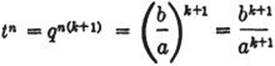 . Hence
(8) 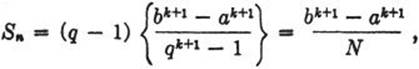
where
![]()
Thus far n has been a fixed number. Now we shall let n increase, and determine the limit of N. As n increases, the nth root  will tend to 1 (see p. 323), and therefore both numerator and denominator of N will tend to zero, which makes caution necessary. Suppose first that k is a positive integer; then the division by q – 1 can be carried out, and we obtain (see p. 13) N = qk + qk-1 + · · · + q + 1. If now n increases, q tends to 1 and hence q2 q3, · · ·, qk will also tend to 1, so that N approaches k + 1. But this shows that Sn tends to
 ![]() as was to be proved.
as was to be proved.
Exercise: Prove that for any rational k ≠ – 1 the same limit formula, N → k + 1, and therefore the result (7), remains valid. First give the proof, according to our model, for negative integers k. Then, if k = u/v, write q1/v = s and
![]()
If n increases, both s and q tend to 1, and therefore the two quotients on the right hand side tend to u + v and v respectively, which yields again ![]() for the limit of N.
for the limit of N.
In §5 we shall see how this lengthy and somewhat artificial discussion may be replaced by the simpler and more powerful methods of the calculus.
Exercises: 1) Check the preceding integration of xk for the cases k = ½, –½, 2, –2, 3, –3.
2) Find the values of the integrals:

3) Find the values of the integrals:
![]()
(Hint: Consider the graphs of the functions under the integral sign, take into account their symmetry with respect to x = 0, and interpret the integrals as areas.)
*4) Integrate sin x and cos x from 0 to b by substituting Δx = h and using the formulas of page 488.
5) Integrate f(x) = x and f(x) = x2 from 0 to b by subdividing into equal parts and by using in (6a) the values ![]() .
.
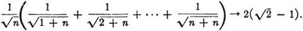
*6) Using the result (7) and the definition of the integral with equal values of Δx prove the limiting relation:
![]()
(Hint: Set ![]() and show that the limit is equal to
and show that the limit is equal to ![]() .)
.)
*7) Prove for n → ∞:
(Hint: Write this sum so that its limit appears as an integral.)
8) Calculate the area of a parabolic segment bounded by an arc P1P2 and the chord P1P2 of a parabola y = ax2 in terms of the coördinates x1 and x2 of the two points.
5. Rules for the “Integral Calculus”
An important step in the development of the calculus was taken when certain general rules were formulated by means of which more involved problems could be reduced to simpler ones and thereby be solved by an almost mechanical procedure. This algorithmic feature is particularly emphasized by Leibniz’ notation. Still, too much concentration on the mechanics of problem solving can degrade the teaching of the calculus into an empty drill.
Some simple rules for integrals follow at once either from the definition (6) or from the geometrical interpretation of integrals as areas.
The integral of the sum of two functions is equal to the sum of the integrals of the two functions. The integral of a constant c times a function f(x) is c times the integral of f(x). These two rules combined are expressed in the formula
(9) 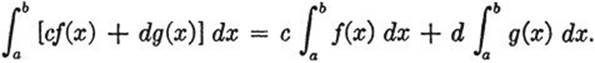
The proof follows immediately from the definition of the integral as the limit of the finite sum (5), since the corresponding formula for a sum Sn is obviously true. The rule extends immediately to sums of more than two functions.
As an example of the use of this rule we consider a polynomial,
f(x) = a0 + a1x + a2x2 + · · · + anxn,
where the coefficients ao, a1, · · ·, an are constants. To form the integral of f(x) from a to b, we proceed termwise, according to the rule. Using formula (7) we find
![]()
Another rule, obvious both from the analytic definition and the geometric interpretation, is given by the formula:
(10) ![]()
Furthermore, it is clear that the integral becomes zero if b is equal to a. The rule of page 405,
(11) ![]()
is in agreement with the last two rules, since it corresponds to (10) for c = a.
Sometimes it is convenient to use the fact that the value of the integral in no way depends upon the particular name x chosen for the independent variable in f(x); for example
![]()
For a mere change in the name of the coordinates in the system to which the graph of the function refers does not alter the area under the curve. The same remark applies even if we make certain changes in the coordinate system itself. For example, let us shift the origin to the right by one unit from O to O′, as in Figure 265, so that x is replaced by a new coördinate x′ such that x = 1 + x′. A curve with the equation y = f(x) will have in the new coördinate system the equation y = f(1 + x′). (E.g. y = 1/x = 1/(1+x′)·) A given area A under this curve, say between x = 1 and x = b, is, in the new coördinate system, the area under the arch between x′ = 0 and x′ = b – 1. Thus we have
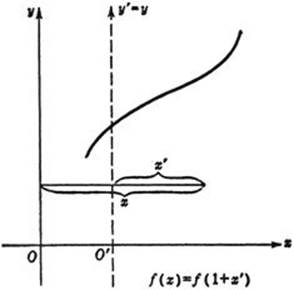
Fig. 265 Shifting of y-axis.
![]()
or, changing the name x′ to u,
(12) ![]()
For example,
(12a) ![]()
and for the function f(x) = xk,
(12b) ![]()
Similarly,
(12c) ![]()
Since the left side of (12c) is equal to ![]() , we obtain
, we obtain
(12d) ![]()
Exercises: 1) Calculate the integral of 1 + x + x2 + · · · + xn from 0 to b.
2) For n > 0 prove that the integral of (1 + x)n from –1 to z is equal to
![]()
3) Show that the integral from 0 to 1 of xn sin x is smaller than 1/(n + 1). (Hint: The latter value is the integral of xn).
4) Prove directly and by use of the binomial theorem that the integral from ![]() .
.
Finally we mention two important rules which have the form of inequalities. These rules permit rough, but useful, appraisals of the values of integrals.
We suppose that b > a and that the values of f(x) in the interval nowhere exceed those of another function g(x). Then we have
(13) ![]()
as is immediately clear either from Figure 266 or from the analytic definition of the integral. In particular, if g(x) = M is a constant not exceeded by the values of f(x), we have ![]() It follows that
It follows that
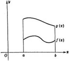
Fig. 266. Comparison of integrals.
(14) ![]()
If f(x) is not negative, then f(x) = | f(x) |. If f(x) < 0, then | f(x) | > f(x). Hence, setting g(x) = | f(x) | in (13), we obtain the useful formula
(15) ![]()
Since | –f(x) | = | f(x) |, we also have
![]()
which, together with (15), yields the somewhat stronger inequality
(16) ![]()