What Is Mathematics? An Elementary Approach to Ideas and Methods, 2nd Edition (1996)

§10. STEINER’S PROBLEM

Steiner’s problem (p. 354) concerns a triangle ABC, and it requires us to find a point P that minimizes the total distance PA + PB + PC. The answer, at least when the angles of triangle ABC are all less than 120°, is that P is the unique point such that the lines PA, PB, and PC meet at 120° to each other (pp. 355-6). Steiner’s problem can be generalized to the street network problem, which asks for the shortest network of lines (streets) joining a given set of points (towns) to each other (p. 359). It has given rise to a fascinating conjecture, only recently proved.

Suppose we wish to find a network of lines that will connect a set of towns. One way to do this is to use a so-called spanning network, which uses only the straight lines joining pairs of towns. Another is to use a Steiner network, in which extra towns are permitted, such that the lines running into them meet at 120° angles. Let the length of the shortest spanning network for a given set of towns be called the spanning length, and let the length of the shortest Steiner network be the Steiner length. The problem of finding the Steiner length is discussed by Courant and Robbins (p. 359) under the title “Street Network Problem.” Obviously the Steiner length is less than or equal to the spanning length. How much smaller can it get?

Suppose, for example, that there are three towns at the vertices of an equilateral triangle of side 1 unit. Fig. 295 shows the shortest Steiner network and the shortest spanning network. The new point introduced in the center is called a Steiner point: in general, a Steiner point is one at which three lines (joining it to other points in the set of towns) meet at angles of 120°. The spanning length is 2 and the Steiner length is √3. In this case, the ratio between the Steiner length and the spanning length is √3/2 = 0.866, and the saving in length obtained by using the shortest Steiner network rather than the shortest spanning network is about 13.34%.

In 1968, Edgar Gilbert and Henry Pollak conjectured that no matter how the towns are initially located, the Steiner length never falls short of the spanning length by more than 13.34%. Equivalently,

(7) 

for any set of towns. This statement has become known as the Steiner ratio conjecture. After considerable effort it was finally proved by Ding Zhu Du and Frank Hwang in 1991: we describe their approach once we have set up the necessary background.

Finding the spanning length is a simple computation, even for a huge number of towns. It is solved by the greedy algorithm: start with the shortest connecting line you can find, and at each stage thereafter add on the shortest remaining line that does not complete a closed loop, until every town is included. Finding the Steiner length is nowhere near as easy. You cannot just take all possible triples of towns, find their Steiner points, and look for the shortest network that joins the towns and meets either at towns or at these particular Steiner points. For example, suppose there are six towns arranged at the corners of two adjacent squares, as in Fig. 296 One possible Steiner tree is shown in Fig. 296a: it is found by solving the problem for a square of four towns first, and then linking in the two remaining towns via their Steiner point with one that is already hooked in. However, the shortest Steiner tree is that shown in Fig. 296b. The grey squares are included only to indicate where the towns are placed.

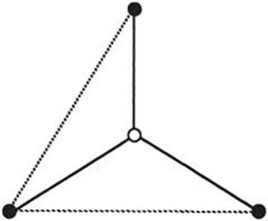
Fig. 295. Shortest Steiner network (solid lines) and shortest spanning network (dotted lines) for three towns in an equilateral triangle.

You cannot build up shortest Steiner trees piecemeal. The correct generalization of Steiner point to a set of many towns is any point at which links can meet at 120°. For as simple an example as four towns at the vertices of a square, these points are not Steiner points of any subset of three towns (Fig. 297). There are infinitely many points in the plane, and even though most of them are probably irrelevant, it is not obvious that any algorithms exist. In fact they do; the first was invented by Z. A. Melzak, but in practice his method becomes unwieldy even for moderate numbers of towns. It has since been improved, but not dramatically.

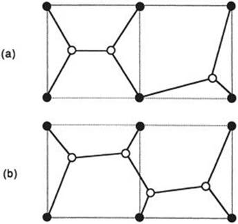
Fig. 296. (a) Combining Steiner trees for a square and an isosceles right triangle. (b) A shorter Steiner tree for the same set of towns.

We now know that there are good reasons why these algorithms are inefficient. The growing use of computers has led to the development of a new branch of mathematics, Algorithmic Complexity Theory. This studies not just algorithms—methods for solving problems—but how efficient those algorithms are. Given a problem involving some number n of objects (here towns), how fast does the running time of the solution grow as n grows? If the running time grows no faster than a constant multiple of a fixed power of n, such as 5n² or 1066n⁴, then the algorithm is said to run in polynomial time, and the problem is considered to be “easy.” Usually this means that the algorithm is practical (but it will not be if the constant is absolutely huge). If the running time grows non-polynomially—faster than any constant multiple of powers of n, for instance exponentially, like 2ⁿ or 10ⁿ—then the problem has non-polynomial running time and is “hard.” Usually this means that the algorithm is totally impractical. In between polynomial time and exponential time is a wilderness of “fairly easy” or “moderately hard” problems, where practicality is more a matter of experience.

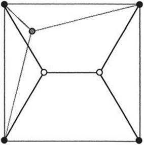
Fig. 297. Steiner points (white) for four towns in a square (black) are different from the Steiner points of a subset of three towns (grey).

For instance, adding two n-digit numbers requires at most 2n one-digit additions, including carries, so the time taken is bounded by a constant multiple (namely 2) of the first power of n. Long multiplication of two such numbers involves about n² one-digit multiplications and no more than 2n² additions, or 3n² operations on digits, so now the bound involves only the second power of n. The opinions of schoolchildren notwithstanding, these problems are therefore “easy.” In contrast, consider the Traveling Salesman Problem: find the shortest route that takes a salesman through a given set of cities. If there are n cities then the number of routes that we have to consider is n! = n(n – 1)(n – 2)… 3.2.1 which grows faster than any power of n. So case-by-case enumeration is hopelessly inefficient.

Oddly enough, the big problem in Algorithmic Complexity Theory is to prove that the subject actually exists. That is, to prove that some “interesting” problem really is hard. The difficulty is that it is easy to prove a problem is easy, but hard to prove that it is hard! To show a problem is easy, you just exhibit an algorithm that solves it in polynomial time. It does not have to be the best or the cleverest: any will do. But to prove that a problem is hard, it is not enough to exhibit some algorithm with non-polynomial running time. Maybe you chose the wrong algorithm; maybe there is a better one which does run in polynomial time. In order to rule that possibility out, you have to find some mathematical way to consider all possible algorithms for the problem and show that none of them runs in polynomial time. And that is extremely difficult.

There are lots of candidates for hard problems—the traveling salesman problem, the bin-packing problem (how can you best fit a set of items of given sizes into a set of sacks of given sizes?), and the knapsack problem (given a fixed size sack and many objects, does any set of objects fill the bag exactly?). So far nobody has managed to prove any of them are hard. However, in 1971 Stephen Cook of the University of Toronto showed that if you can prove that any one problem in this candidate group really is hard, then they all are. Roughly speaking, you can “code” any one of them to become a special case of one of the others: they sink or swim together. These problems are called NP-complete, where NP stands for non-polynomial. Everyone believes that NP-complete problems really are hard, but this has never been proved.

NP-completeness relates to the Steiner problem because Ronald Graham, Michael Garey and David Johnson have proved that the problem of computing the Steiner length is NP-complete. That is, any efficient algorithm to find the precise Steiner length for any set of towns would automatically lead to efficient solutions to all sorts of computational problems that are widely believed not to possess such solutions.

The Steiner ratio conjecture (7) is therefore important, because it proves you can replace a hard problem by an easy one without losing very much. Gilbert and Pollak had quite a lot of positive evidence when they stated that conjecture. In particular they could prove that something weaker must be true: the ratio of Steiner length to spanning length is always at least 0.5. By 1990 various people had performed heroic calculations to verify the conjecture completely for networks of 4, 5, and 6 towns. For general arrangements of as many towns as you like, they also pushed up the limits on the ratio from 0.5 to 0.57, 0.74, and 0.8. Around 1990 Graham and Fang Chung raised it to 0.824, in a computation that they described as “really horrible—it was clear it was the wrong approach.”

To make further progress possible, the horrible calculations had to be simplified. Du and Hwang found an approach that is so much better, it does away with the horrible calculations completely. The basic question is how to get equilateral triangles in on the act. There is a big gap between the triangle example in Fig. 295, which sets the bound on the ratio, and a general system of towns, which is supposed to obey the same bound. How can this No Man’s Land be crossed? There is a kind of halfway house. Imagine the plane tiled with identical equilateral triangles, in a triangular lattice (Fig. 298). Put towns only at the corners of the tiles. It turns out that the only Steiner points that need be considered are the centers of the tiles. In short, you have a lot of control, not just on computations, but on theoretical analyses.

Of course, not every set of towns conveniently lies on a triangular lattice. Du and Hwang’s insight is that the crucial ones do. Again the proof is indirect, by contradiction. Suppose the conjecture is false. Then there must exist a counterexample: some set of towns for which the ratio is less than √3/2. Du and Hwang show that if a counterexample to the conjecture exists then there must be one for which all the towns lie on a triangular lattice. This introduces an element of regularity into the problem, and it is then relatively simple to complete the proof.

In order to prove this lattice property they reformulate the conjecture as a problem in game theory, where players compete and try to limit the gains made by their opponents. Game theory was invented by John von Neumann and Oskar Morgenstern in their classic Theory of Games and Economic Behavior of 1947. In the Du-Hwang version of the Steiner ratio conjecture, one player selects the general “shape” of the Steiner tree, and the other picks the shortest one of that shape that they can find. Du and Hwang deduce the existence of a lattice counterexample by observing that the payoff for their game has a special “convexity” property.