Discrete Fractional Calculus (2015)
1. Basic Difference Calculus
1.9. Vector Difference Equations
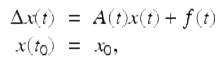
In this section, we will examine the properties of the linear vector difference equation with variable coefficients
![]()
(1.40)
and the corresponding homogeneous system
![]()
(1.41)
where ![]() and the real n × 1 matrix function A(t) will be assumed to be a regressive matrix function on
and the real n × 1 matrix function A(t) will be assumed to be a regressive matrix function on ![]() (that is I + A(t) is nonsingular for all
(that is I + A(t) is nonsingular for all ![]() ). With these assumptions, it is easy to show that for any
). With these assumptions, it is easy to show that for any ![]() the initial value problem
the initial value problem
where ![]() is a given n × 1 constant vector, has a unique solution on
is a given n × 1 constant vector, has a unique solution on ![]() To solve the nonhomogeneous difference equation (1.40) we will see that we first want to be able to solve the corresponding homogeneous difference equation (1.41). The matrix equation analogue of the homogeneous vector difference equation (1.41) is
To solve the nonhomogeneous difference equation (1.40) we will see that we first want to be able to solve the corresponding homogeneous difference equation (1.41). The matrix equation analogue of the homogeneous vector difference equation (1.41) is
![]()
(1.42)
where U(t) is an n × n matrix function. Note that U(t) is a solution of (1.42) if and only if each of its column vectors is a solution of (1.41). From the uniqueness of solutions to IVPs for the vector equation (1.40) we have that the matrix IVP
![]()
where ![]() and U 0 is a given n × n constant matrix has a unique solution on
and U 0 is a given n × n constant matrix has a unique solution on ![]()
Theorem 1.78.
Assume A(t) is a regressive matrix function on ![]() . If
. If ![]() is a solution of (1.42) , then either det
is a solution of (1.42) , then either det ![]() for all
for all ![]() or det
or det ![]() for all
for all ![]() .
.
Proof.
Since ![]() is a solution of (1.42) on
is a solution of (1.42) on ![]() ,
,
![]()
Therefore,
![]()
(1.43)
for all ![]() . Now either
. Now either ![]() or
or ![]() . Since det [I + A(t)] ≠ 0 for all
. Since det [I + A(t)] ≠ 0 for all ![]() , we have by (1.43) that if
, we have by (1.43) that if ![]() , then
, then ![]() for all
for all ![]() , while if
, while if ![]() , then
, then ![]() for all
for all ![]() . □
. □
Definition 1.79.
We say that ![]() is a fundamental matrix of the vector difference equation (1.41) provided
is a fundamental matrix of the vector difference equation (1.41) provided ![]() is a solution of the matrix equation (1.42) and
is a solution of the matrix equation (1.42) and ![]() for
for ![]() .
.
Definition 1.80.
If A is a regressive matrix function on ![]() , then we define the matrix exponential function, e A (t, t 0), based at
, then we define the matrix exponential function, e A (t, t 0), based at ![]() to be the unique solution of the matrix IVP
to be the unique solution of the matrix IVP
![]()
From Exercise 1.71 we have that ![]() is a fundamental matrix of
is a fundamental matrix of ![]() if and only if its columns are n linearly independent solutions of the vector equation
if and only if its columns are n linearly independent solutions of the vector equation ![]() on
on ![]() . To find a formula for the matrix exponential function, e A (t, t 0), we want to solve the IVP
. To find a formula for the matrix exponential function, e A (t, t 0), we want to solve the IVP
![]()
Iterating this equation we get
![$$\displaystyle{e_{A}(t,t_{0}) = \left \{\begin{array}{@{}l@{\quad }l@{}} \;^{{\ast}}\prod _{ s=t_{0}}^{t-1}[I + A(s)],\quad t \in \mathbb{N}_{ t_{0}} \quad \\ \quad \prod _{s=t}^{t_{0}-1}[I + A(s)]^{-1},\quad t \in \mathbb{N}_{a}^{t_{0}-1},\quad \end{array} \right.}$$](fractional.files/image570.png)
where it is understood that ![]() and for
and for ![]()
![$$\displaystyle{\;^{{\ast}}\prod _{ s=t_{0}}^{t-1}[I + A(s)]:= [I + A(t - 1)][I + A(t - 2)]\cdots [I + A(t_{ 0})].}$$](fractional.files/image573.png)
Example 1.81.
If A is an n × n constant matrix and I + A is invertible, then
![]()
Similar to the proof of Theorem 1.16 one can prove (Exercise 1.73) the following theorem.
Theorem 1.82.
The set of all n × n regressive matrix functions on ![]() with the addition, ⊕ defined by
with the addition, ⊕ defined by
![]()
is a group. Furthermore, the additive inverse of a regressive matrix function A defined on ![]() is given by
is given by
![]()
In the next theorem we give several properties of the matrix exponential. To prove part (vii) of the this theorem we will use the following lemma.
Lemma 1.83.
Assume Y (t) and ![]() are invertible matrices. Then
are invertible matrices. Then
![]()
Proof.
Taking the difference of both sides of Y (t)Y −1(t) = I we get that
![]()
Solving this last equation for ![]() we get that
we get that
![]()
Similarly, one can use Y −1(t)Y (t) = I to get that
![]()
□
Theorem 1.84.
Assume A and B are regressive matrix functions on ![]() and
and ![]() Then the following hold:
Then the following hold:
(i)
![]()
(ii)
e A (s,s) = I;
(iii)
![]() for
for ![]()
(iv)
e A (t,s) is a fundamental matrix of (1.41) ;
(v)
![]()
(vi)
(semigroup property) e A (t,r)e A (r,s) = e A (t,s) holds for ![]()
(vii)
![]()
(viii)
![]() where A ∗ denotes the conjugate transpose of the matrix A;
where A ∗ denotes the conjugate transpose of the matrix A;
(ix)
B(t)e A (t,t 0 ) = e A (t,t 0 )B(t), if A(t) and B(τ) commute for all ![]()
(x)
e A (t,s)e B (t,s) = e A⊕B (t,s), if A(t) and B(τ) commute for all ![]() .
.
Proof.
Note that (i) and (ii) follow from the definition of the matrix exponential. Part (iii) follows from Theorem 1.78 and part (ii). Parts (i) and (iii) imply part (iv) holds. Since ![]() , we have that
, we have that
![]()
and hence (v) holds. To see that the semigroup property (vi) holds, fix ![]() and set
and set ![]() Then
Then
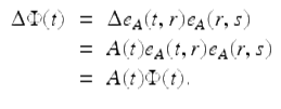
Next we show that ![]() First note that if r = s, then
First note that if r = s, then ![]() . Hence we can assume that s ≠ r. For the case r > s ≥ a, we have that
. Hence we can assume that s ≠ r. For the case r > s ≥ a, we have that
![$$\displaystyle\begin{array}{rcl} \Phi (s)& =& e_{A}(s,r)e_{A}(r,s) = \left (\prod _{\tau =s}^{r-1}[I + A(\tau )]^{-1}\right )\left (\;^{{\ast}}\prod _{ \tau =s}^{r-1}[I + A(\tau )]\right ) {}\\ & =& [I + A(s)]^{-1}\cdots [I + A(r - 1)]^{-1}[I + A(r - 1)]\cdots [I + A(s)] = I. {}\\ \end{array}$$](fractional.files/image600.png)
Similarly, for the case s > r ≥ a one can show that ![]() Hence, by the uniqueness of solutions for IVPs we get that e A (t, r)e A (r, s) = e A (t, s). To see that (vii) holds, fix
Hence, by the uniqueness of solutions for IVPs we get that e A (t, r)e A (r, s) = e A (t, s). To see that (vii) holds, fix ![]() and let
and let
![]()
Then
![$$\displaystyle\begin{array}{rcl} \Delta Y (t)& =& \left [\Delta e_{A}^{-1}(t,s)\right ]^{{\ast}} {}\\ & =& -\left [e_{A}^{-1}(\sigma (t),s)\Delta e_{ A}(t,s)e_{A}^{-1}(t,s)\right ]^{{\ast}} {}\\ & =& -\left [e_{A}^{-1}(\sigma (t),s)A(t)\right ]^{{\ast}} {}\\ & =& -\left [\left ([I + A(t)]e_{A}(t,s)\right )^{-1}A(t)\right ]^{{\ast}} {}\\ & =& -\left [e_{A}^{-1}(t,s)[I + A(t)]^{-1}A(t)\right ]^{{\ast}} {}\\ & =& -A^{{\ast}}(t)[I + A^{{\ast}}(t)]^{-1}\left [e_{ A}^{-1}(t,s)\right ]^{{\ast}} {}\\ & =& (\ominus A^{{\ast}})(t)Y (t). {}\\ \end{array}$$](fractional.files/image604.png)
Since ![]() and
and ![]() satisfy the same matrix IVP we get
satisfy the same matrix IVP we get
![]()
Taking the conjugate transpose of both sides of this last equation we get that part (vii) holds. The proof of (viii) is Exercise 1.78 and the proof of (ix) is Exercise 1.79.
To see that (x) holds, let ![]() ,
, ![]() . Then by the product rule
. Then by the product rule
![$$\displaystyle\begin{array}{rcl} \Delta \Phi (t)& =& \Delta \left [e_{A}(t,s)e_{B}(t,s)\right ] {}\\ & =& e_{A}(\sigma (t),s)\Delta e_{B}(t,s) + \Delta e_{A}(t,s)e_{B}(t,s) {}\\ & =& [1 + A(t)]e_{A}(t,s)B(t)e_{B}(t,s) + A(t)e_{A}(t,s)e_{B}(t,s) {}\\ & =& [A(t) + B(t) + A(t)B(t)]e_{A}(t,s)e_{B}(t,s) {}\\ & =& [(A \oplus B)(t)]\Phi (t) {}\\ \end{array}$$](fractional.files/image609.png)
for ![]() . Since
. Since ![]() , we have that
, we have that ![]() and e A⊕B (t, s) satisfy the same matrix IVP. Hence, by the uniqueness theorem for solutions of matrix IVPs we get the desired result e A (t, s)e B (t, s) = e A⊕B (t, s). □
and e A⊕B (t, s) satisfy the same matrix IVP. Hence, by the uniqueness theorem for solutions of matrix IVPs we get the desired result e A (t, s)e B (t, s) = e A⊕B (t, s). □
Now for any nonsingular matrix U 0, the solution U(t) of (1.42) with U(t 0) = U 0 is a fundamental matrix of (1.41), so there are always infinitely many fundamental matrices of (1.41). In particular, if A is a regressive matrix function on ![]() , then
, then ![]() is a fundamental matrix of the vector equation
is a fundamental matrix of the vector equation ![]()
The following theorem characterizes fundamental matrices for (1.41).
Theorem 1.85.
If ![]() is a fundamental matrix for (1.41) , then
is a fundamental matrix for (1.41) , then ![]() is another fundamental matrix if and only if there is a nonsingular constant matrix C such that
is another fundamental matrix if and only if there is a nonsingular constant matrix C such that
![]()
for ![]() .
.
Proof.
Let ![]() , where
, where ![]() is a fundamental matrix of (1.41) and C is nonsingular constant matrix. Then
is a fundamental matrix of (1.41) and C is nonsingular constant matrix. Then ![]() is nonsingular for all
is nonsingular for all ![]() , and
, and

Therefore ![]() is a fundamental matrix of (1.41).
is a fundamental matrix of (1.41).
Conversely, assume ![]() and
and ![]() are fundamental matrices of (1.41). For some
are fundamental matrices of (1.41). For some ![]() , let
, let
![]()
Then ![]() and
and ![]() are both solutions of (1.42) satisfying the same initial condition at t 0. By uniqueness,
are both solutions of (1.42) satisfying the same initial condition at t 0. By uniqueness,
![]()
for all ![]() . □
. □
The proof of the following theorem is similar to that of Theorem 1.85 and is left as an exercise (Exercise 1.68).
Theorem 1.86.
If ![]() is a fundamental matrix of (1.41) , then the general solution of (1.41) is given by
is a fundamental matrix of (1.41) , then the general solution of (1.41) is given by
![]()
where c is an arbitrary constant column vector.
Hence we see to solve the vector equation (1.41) we just need to find the fundamental matrix ![]() We will set off to prove the Putzer algorithm (Theorem 1.88) which will give us a nice formula e A (t, 0), for
We will set off to prove the Putzer algorithm (Theorem 1.88) which will give us a nice formula e A (t, 0), for ![]() when A is a constant n × n matrix. In the proof of this theorem we will use the Cayley–Hamilton Theorem which states that every square constant matrix satisfies its own characteristic equation. We now give an example to illustrate this important theorem.
when A is a constant n × n matrix. In the proof of this theorem we will use the Cayley–Hamilton Theorem which states that every square constant matrix satisfies its own characteristic equation. We now give an example to illustrate this important theorem.
Example 1.87.
Show directly that the matrix
![$$\displaystyle{A = \left [\begin{array}{*{10}c} 2&-1\\ 3 &-4 \end{array} \right ]}$$](fractional.files/image624.png)
satisfies its own characteristic equation. The characteristic equation of A is
![]()
Then
![$$\displaystyle\begin{array}{rcl} A^{2} + 2A - 5I& =& \left [\begin{array}{*{10}c} \;\;\;1 & 2 \\ -6&13 \end{array} \right ] + \left [\begin{array}{*{10}c} 4&-2\\ 6 &-8 \end{array} \right ] -\left [\begin{array}{*{10}c} 5&0\\ 0 &5 \end{array} \right ] {}\\ & =& \left [\begin{array}{*{10}c} 0&0\\ 0 &0 \end{array} \right ] {}\\ \end{array}$$](fractional.files/image626.png)
and so A does satisfy its own characteristic equation.
The proof of the next theorem is motivated by the fact that by the Cayley–Hamilton Theorem an n by n constant matrix A can be written as a linear combination of the matrices I, A, A 2, ![]() , A n−1 and therefore every nonnegative integer power A t of A can also be written as a linear combination of I, A, A 2,
, A n−1 and therefore every nonnegative integer power A t of A can also be written as a linear combination of I, A, A 2, ![]() , A n−1.
, A n−1.
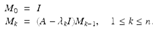
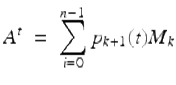
Theorem 1.88 (Putzer’s Algorithm).
Let ![]() be the (not necessarily distinct) eigenvalues of the constant n by n matrix A, with each eigenvalue repeated as many times as its multiplicity. Define the matrices M k , 0 ≤ k ≤ n, recursively by
be the (not necessarily distinct) eigenvalues of the constant n by n matrix A, with each eigenvalue repeated as many times as its multiplicity. Define the matrices M k , 0 ≤ k ≤ n, recursively by
Then
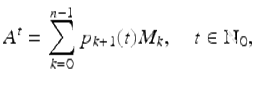
where the p k (t), 1 ≤ k ≤ n are chosen so that
![$$\displaystyle{ \left [\begin{array}{*{10}c} p_{1}(t + 1) \\ p_{2}(t + 1)\\ \vdots \\ p_{n}(t + 1) \end{array} \right ]\ \ = \left [\begin{array}{*{10}c} \lambda _{1} & 0 &0&\cdots & 0 \\ 1& \lambda _{2} & 0&\cdots & 0 \\ 0& 1 & \lambda _{3} & \cdots & 0\\ \vdots & \ddots & \ddots & \ddots & \vdots \\ 0&\cdots &0& 1 &\lambda _{n} \end{array} \right ]\left [\begin{array}{*{10}c} p_{1}(t) \\ p_{2}(t)\\ \vdots \\ p_{n}(t) \end{array} \right ] }$$](fractional.files/image631.png)
(1.44)
and
![$$\displaystyle{ \left [\begin{array}{*{10}c} p_{1}(0) \\ p_{2}(0)\\ \vdots \\ p_{n}(0) \end{array} \right ] = \left [\begin{array}{*{10}c} 1\\ 0\\ \vdots \\ 0 \end{array} \right ]. }$$](fractional.files/image632.png)
(1.45)
Proof.
Let the matrices M k , 0 ≤ k ≤ n be defined as in the statement of this theorem. Since for each fixed t ≥ 0, A t is a linear combination of I, A, A 2, ![]() , A n−1, we also have that for each fixed t, A t is a linear combination of M 0, M 1, M 2,
, A n−1, we also have that for each fixed t, A t is a linear combination of M 0, M 1, M 2, ![]() , M n−1, that is
, M n−1, that is
for t ≥ 0. It remains to show that the p k ’s are as in the statement of this theorem. Since A t+1 = A ⋅ A t , we have that
![$$\displaystyle\begin{array}{rcl} \sum _{k=0}^{n-1}p_{ k+1}(t + 1)M_{k}& =& A\sum _{k=0}^{n-1}p_{ k+1}(t)M_{k} \\ & =& \sum _{k=0}^{n-1}p_{ k+1}(t)\left [AM_{k}\right ] \\ & =& \sum _{k=0}^{n-1}p_{ k+1}(t)\left [M_{k+1} +\lambda _{k+1}M_{k}\right ] \\ & =& \sum _{k=0}^{n-1}p_{ k+1}(t)M_{k+1} +\sum _{ k=0}^{n-1}\lambda _{ k+1}p_{k+1}(t)M_{k} \\ & =& \sum _{k=1}^{n-1}p_{ k}(t)M_{k} +\sum _{ k=0}^{n-1}p_{ k+1}(t)\lambda _{k+1}M_{k}, \\ & =& \lambda _{1}p_{1}(t)M_{0} +\sum _{ k=1}^{n-1}\left [p_{ k}(t) +\lambda _{k+1}p_{k+1}(t)\right ]M_{k},{}\end{array}$$](fractional.files/image634.png)
(1.46)
where in the second to the last step we have replaced k by k − 1 in the first sum and used the fact that (by the Cayley–Hamilton Theorem) M n = 0. Note that equation (1.46) is satisfied if p k (t), ![]() are chosen to satisfy the system (1.44). Since
are chosen to satisfy the system (1.44). Since ![]() , we must have (1.45) is satisfied. □
, we must have (1.45) is satisfied. □
The following example shows how we can use the Putzer algorithm to find the exponential function e A (t, 0) when A is a constant matrix. This method is called finding the matrix exponential e A (t, 0) using the Putzer algorithm.
Example 1.89.
Use the Putzer algorithm (Theorem 1.88) to find e A (t, 0), ![]() , where
, where
![$$\displaystyle{A:= \left [\begin{array}{*{10}c} 1&2\\ 1 &\;2 \end{array} \right ].}$$](fractional.files/image637.png)
Note ![]() . So to find e A (t, 0) we just need to find B t where
. So to find e A (t, 0) we just need to find B t where
![$$\displaystyle{B:= I+A = \left [\begin{array}{*{10}c} 2&2\\ 1 &3 \end{array} \right ].}$$](fractional.files/image639.png)
We now apply Putzer’s algorithm (Theorem 1.88) to find B t . The characteristic equation for B is given by ![]() . Hence the eigenvalues of B are given by
. Hence the eigenvalues of B are given by ![]()
![]() . It follows that M 0 = I and
. It follows that M 0 = I and
![$$\displaystyle{M_{1} = B-\lambda _{1}I = \left [\begin{array}{*{10}c} 1&2\\ 1 &2 \end{array} \right ].}$$](fractional.files/image643.png)
To find p 1(t) we now solve the IVP
![]()
It follows that p 1(t) = 1. Next to find p 2(t) we solve the IVP
![]()
This gives us the IVP
![]()
Using the variation of constants formula in Theorem 1.68 we get
![$$\displaystyle\begin{array}{rcl} p_{2}(t)& =& \int _{0}^{t}e_{ 3}(t,\sigma (s))\Delta s {}\\ & =& \int _{0}^{t}e_{ \ominus 3}(\sigma (s),t)\Delta s {}\\ & =& \int _{0}^{t}[1 + \ominus 3]e_{ \ominus 3}(s,t)\Delta s {}\\ & =& \frac{1} {4}\int _{0}^{t}e_{ \ominus 3}(s,t)\Delta s {}\\ & =& -\frac{1} {3}e_{\ominus 3}(s,t)\vert _{s=0}^{s=t} {}\\ & =& -\frac{1} {3}e_{\ominus 3}(t,t) + \frac{1} {3}e_{\ominus 3}(0,t) {}\\ & =& -\frac{1} {3} + \frac{1} {3}e_{3}(t,0) {}\\ & =& -\frac{1} {3} + \frac{1} {3}4^{t}. {}\\ \end{array}$$](fractional.files/image647.png)
It follows that
![$$\displaystyle\begin{array}{rcl} e_{A}(t,0)& =& p_{1}(t)M_{0} + p_{2}(t)M_{1} {}\\ & =& \left [\begin{array}{*{10}c} 1&0\\ 0 &1 \end{array} \right ] +\bigg (-\frac{1} {3} + \frac{1} {3}4^{t}\bigg)\left [\begin{array}{*{10}c} 1&2 \\ 1&2 \end{array} \right ] {}\\ & =& \frac{1} {3}\left [\begin{array}{*{10}c} \;\;2 + 4^{t} &-2 + 2 \cdot 4^{t} \\ -1 + 4^{t}& \;\;1 + 2 \cdot 4^{t} \end{array} \right ]. {}\\ \end{array}$$](fractional.files/image648.png)
It follows from this that
![$$\displaystyle{y(t) = c_{1}\left [\begin{array}{*{10}c} \;\;2 + 4^{t} \\ -1 + 4^{t} \end{array} \right ]+c_{2}\left [\begin{array}{*{10}c} -2 + 2 \cdot 4^{t} \\ \;\;1 + 2 \cdot 4^{t} \end{array} \right ]}$$](fractional.files/image649.png)
is a general solution of
![$$\displaystyle{\Delta y(t) = \left [\begin{array}{*{10}c} 1&2\\ 1 &\;2 \end{array} \right ]y(t),\quad t \in \mathbb{N}_{0}.}$$](fractional.files/image650.png)
Example 1.90.
Use Putzer’s algorithm for finding the matrix exponential e A (t, 0) to solve the vector equation
![]()
where A is the regressive matrix given by
![$$\displaystyle{A = \left [\begin{array}{*{10}c} \;\;1 &1\\ -1 &3 \end{array} \right ].}$$](fractional.files/image652.png)
Let B: = I + A, then e A (t, 0) = [I + A] t = B t , where
![$$\displaystyle{B = \left [\begin{array}{*{10}c} \;\;2 &1\\ -1 &4 \end{array} \right ].}$$](fractional.files/image653.png)
The characteristic equation of the constant matrix B is given by
![]()
and so the characteristic values are ![]() It follows that
It follows that
![$$\displaystyle{M_{0} = I = \left [\begin{array}{*{10}c} 1&0\\ 0 &1 \end{array} \right ]\quad \mbox{ and}\quad M_{1} = \left (B - 3I\right )M_{0} = \left [\begin{array}{*{10}c} -1&1\\ -1 &1 \end{array} \right ].}$$](fractional.files/image656.png)
Next we solve the IVP
![$$\displaystyle{p(t+1) = \left [\begin{array}{*{10}c} \;3&0\\ 1 &3 \end{array} \right ]p(t),\quad p(0) = \left [\begin{array}{*{10}c} 1\\ 0 \end{array} \right ].}$$](fractional.files/image657.png)
Hence p 1(t) solves the IVP
![]()
Since ![]() p 1(0) = 1, we have that p 1(t) = e 2(t, 0) = 3 t . Also p 2(t) solves the IVP
p 1(0) = 1, we have that p 1(t) = e 2(t, 0) = 3 t . Also p 2(t) solves the IVP
![]()
It follows that p 2(t) solves the IVP
![]()
Using the variation of constants formula in Theorem 1.68 we get that
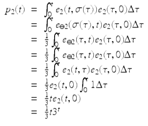
Hence by Putzer’s algorithm
![$$\displaystyle\begin{array}{rcl} e_{A}(t,0)& =& B^{t} {}\\ & =& p_{1}(t)M_{0} + p_{2}(t)M_{1} {}\\ & =& 3^{t}\left [\begin{array}{*{10}c} 1&0 \\ 0&1 \end{array} \right ] + \frac{1} {3}t3^{t}\left [\begin{array}{*{10}c} -1&1 \\ -1&1 \end{array} \right ] {}\\ & =& 3^{t}\left [\begin{array}{*{10}c} 1 -\frac{1} {3}t& \frac{1} {3}t \\ -\frac{1} {3}t &1 + \frac{1} {3}t \end{array} \right ]. {}\\ \end{array}$$](fractional.files/image663.png)
Since e A (t, 0) is a fundamental matrix of ![]() , we have by Theorem 1.86 that
, we have by Theorem 1.86 that
![$$\displaystyle\begin{array}{rcl} u(t)& =& 3^{t}\left [\begin{array}{*{10}c} 1 -\frac{1} {3}t& \frac{1} {3}t \\ -\frac{1} {3}t &1 + \frac{1} {3}t \end{array} \right ]c {}\\ & =& c_{1}3^{t}\left [\begin{array}{*{10}c} 1 -\frac{1} {3}t \\ -\frac{1} {3}t \end{array} \right ] + c_{2}3^{t}\left [\begin{array}{*{10}c} \frac{1} {3}t \\ 1 + \frac{1} {3}t \end{array} \right ]{}\\ \end{array}$$](fractional.files/image665.png)
is a general solution.
Fundamental matrices can be used to solve the nonhomogeneous equation (1.40).
Theorem 1.91 (Variation of Parameters (Constants)).
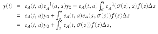
Assume ![]() is a fundamental matrix of (1.41) . Then the unique solution of (1.40) that satisfies the initial condition y(a) = y 0 is given by the variation of parameters formula
is a fundamental matrix of (1.41) . Then the unique solution of (1.40) that satisfies the initial condition y(a) = y 0 is given by the variation of parameters formula
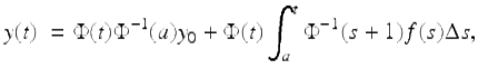
(1.47)
for ![]() .
.
Proof.
Let y(t) be given by (1.47) for ![]() . Using the vector version of the Leibniz formula (1.29), we have
. Using the vector version of the Leibniz formula (1.29), we have
![$$\displaystyle\begin{array}{rcl} \Delta y(t)\ & =& \Delta \Phi (t)\Phi ^{-1}(a)y_{ 0} + \Delta \Phi (t)\int _{a}^{t}\Phi ^{-1}(s + 1)f(s)\Delta s {}\\ & & +\Phi (t + 1)\Phi ^{-1}(t + 1)f(t) {}\\ & =& A(t)\Phi (t)\Phi ^{-1}(a)y_{ 0} + A(t)\Phi (t)\int _{a}^{t}\Phi ^{-1}(s + 1)f(s)\Delta s + f(t) {}\\ & =& A(t)\left [\Phi (t)\Phi ^{-1}(a)y_{ 0} + \Phi (t)\int _{a}^{t}\Phi ^{-1}(s + 1)f(s)\Delta s\right ] + f(t) {}\\ & =& A(t)y(t) + f(t). {}\\ \end{array}$$](fractional.files/image667.png)
Consequently, y(t) defined by (1.47) is a solution of the nonhomogeneous equation, and also we have that y(a) = y 0. □
A special case of the above theorem is the following result.
Theorem 1.92.
Assume A(t) is a regressive matrix function on ![]() and assume
and assume ![]() . Then the unique solution of the IVP
. Then the unique solution of the IVP
![]()
![]()
is given by the variation of constants formula
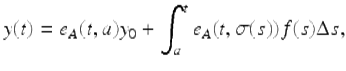
for ![]() .
.
Proof.
Since ![]() is a fundamental matrix of
is a fundamental matrix of ![]() , we have by Theorem 1.91, that the solution of our IVP in the statement of this theorem is given by
, we have by Theorem 1.91, that the solution of our IVP in the statement of this theorem is given by
where in the last two steps we used properties (viii) and (vi) in Theorem 1.84. □
Example 1.93.
Solve the system
![$$\displaystyle\begin{array}{rcl} u(t + 1)& =& \left [\begin{array}{ll} \;\;\;0 &\;\;\;1\\ - 2 & - 3 \end{array} \right ]u(t) + \left (\frac{2} {3}\right )^{t}\left [\begin{array}{l} \;\;\;1 \\ - 2 \end{array} \right ],\quad t \in \mathbb{N}_{0}, {}\\ u(0)& =& \left [\begin{array}{l} 1\\ 1 \end{array} \right ]. {}\\ \end{array}$$](fractional.files/image675.png)
From Exercise 1.72, we can choose
![$$\displaystyle\begin{array}{rcl} \Phi (t)& =& \left [\begin{array}{ll} (-2)^{t} &(-1)^{t} \\ (-2)^{t+1} & (-1)^{t+1} \end{array} \right ] {}\\ & =& (-1)^{t}\left [\begin{array}{ll} \;\;\;2^{t} &\;\;\;1 \\ - 2^{t+1} & - 1 \end{array} \right ].{}\\ \end{array}$$](fractional.files/image676.png)
Then
![$$\displaystyle{\Phi ^{-1}(t) = \frac{(-1)^{t}} {2^{t}} \left [\begin{array}{ll} - 1 & - 1\\ \;\;2^{t+1 } & \;\;2^{t} \end{array} \right ].}$$](fractional.files/image677.png)
From (1.47), we have for t ≥ 0,
![$$\displaystyle\begin{array}{rcl} u(t)& =& (-1)^{t}\left [\begin{array}{ll} \;\;\;2^{t} &\;\;\;1 \\ - 2^{t+1} & - 1 \end{array} \right ]\left (\left [\begin{array}{l} - 2\\ \;\;3 \end{array} \right ] +\sum _{ s=0}^{t-1}\left [\begin{array}{l} -.5(-3)^{-s} \\ \;\;\;0 \end{array} \right ]\right ) {}\\ & =& (-1)^{t}\left [\begin{array}{ll} \;\;\;2^{t} &\;\;\;1 \\ - 2^{t+1} & - 1 \end{array} \right ]\left (\left [\begin{array}{l} - 2\\ \;\;3 \end{array} \right ] + \left [\begin{array}{l}.375((-3)^{-t} - 1) \\ \;\;\;\;\;\quad \quad 0 \end{array} \right ]\right ) {}\\ & =& (-1)^{t}\left [\begin{array}{ll} \;\;\;2^{t} &\;\;\;1 \\ - 2^{t+1} & - 1 \end{array} \right ]\left [\begin{array}{l} -.125((-3)^{1-t} + 19) \\ \quad \quad \quad \quad 3 \end{array} \right ]. {}\\ \end{array}$$](fractional.files/image678.png)