Discrete Fractional Calculus (2015)
1. Basic Difference Calculus
1.11. Floquet Systems
In this section we consider the so-called Floquet system
![]()
(1.55)
where ![]() and
and
![]()
and we assume that A(t) is an n × n matrix function which has minimum positive period p (p is an integer). We say that p is the prime period of A(t). Here are two simple scalar examples that are indicative of the behavior of general Floquet systems.
Example 1.102.
Since a(t): = 2 + (−1) t , ![]() is periodic with prime period p = 2, the equation
is periodic with prime period p = 2, the equation
![]()
(1.56)
is a scalar Floquet system with prime period p = 2. Equation (1.56) can be written in the form
![]()
By Theorem 1.14 the general solution of (1.56) is given by
![]()
where h(t): = 1 + (−1) t , ![]() . It follows from (1.8) that for
. It follows from (1.8) that for ![]()
![$$\displaystyle\begin{array}{rcl} u(t)& =& c\prod _{\tau =0}^{t-1}[1 + h(\tau )] {}\\ & =& c\prod _{\tau =0}^{t-1}[2 + (-1)^{\tau }] {}\\ & =& \left \{\begin{array}{@{}l@{\quad }l@{}} (\sqrt{3})^{t},\quad \quad \mbox{ if $t$ is even} \quad \\ (\sqrt{3})^{t+1},\quad \mbox{ if $t$ is odd}.\quad \end{array} \right.{}\\ \end{array}$$](fractional.files/image765.png)
It is easy to check that the last expression above is also true for negative integers. Define the p = 2 periodic function r by
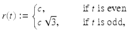
for ![]() and put
and put ![]() . Then we have that all solutions of (1.56) are of the form
. Then we have that all solutions of (1.56) are of the form
![]()
Compare this with formula (1.59) in Floquet’s Theorem 1.105.
In some cases we need b to be a complex number to write the general solution in the form u(t) = r(t)b t as the next example shows.
Example 1.103.
Since a(t): = (−1) t is periodic with prime period p = 2, the equation
![]()
is a scalar Floquet system. The general solution is given by
![]()
We can write this solution in the form
![]()
where

is periodic with period 2 and b = −i. Compare this with the formula (1.59) in Floquet’s Theorem 1.105.
In preparation for the proof of Floquet’s Theorem, we need the following result concerning logarithms of nonsingular matrices.
Lemma 1.104.
Assume C is a nonsingular matrix and p is a positive integer. Then there is a nonsingular matrix B such that
![]()
Proof.
We will prove this theorem only for 2 × 2 matrices. First consider the case where C has two linearly independent eigenvectors. In this case, by the Jordan canonical form theorem, there is a nonsingular matrix Q so that
![]()
where
![$$\displaystyle{J\ =\ \left [\begin{array}{ll} \lambda _{1} & 0 \\ 0&\lambda _{2}\\ \end{array} \right ],}$$](fractional.files/image776.png)
and ![]() ,
, ![]() (
(![]() is possible) are the eigenvalues of C. Now we want to find a matrix B such that
is possible) are the eigenvalues of C. Now we want to find a matrix B such that
![]()
Equivalently, we want to pick B so that
![]()
or
![]()
Then we need to choose B so that
![$$\displaystyle{QBQ^{-1}\ =\ \left [\begin{array}{ll} (\lambda _{1})^{\frac{1} {p} } & \;\;0 \\ \;\;0 &(\lambda _{2})^{\frac{1} {p} } \end{array} \right ],}$$](fractional.files/image783.png)
so
![$$\displaystyle{B\ =\ Q^{-1}\left [\begin{array}{ll} (\lambda _{1})^{\frac{1} {p} } & \;\;0 \\ \;\;0 &(\lambda _{2})^{\frac{1} {p} } \end{array} \right ]Q.}$$](fractional.files/image784.png)
Finally, we consider the case where C has only one linearly independent eigenvector. In this case, by the Jordan canonical form theorem, there is a nonsingular matrix Q so that
![]()
where
![$$\displaystyle{J\ =\ \left [\begin{array}{ll} \lambda _{1} & 1 \\ 0&\lambda _{1}\\ \end{array} \right ],}$$](fractional.files/image786.png)
and ![]() is the eigenvalue of C.
is the eigenvalue of C.
Let’s try to find a matrix B of the form
![$$\displaystyle{ B\ =\ Q^{-1}\left [\begin{array}{ll} a&b \\ 0 &a \end{array} \right ]Q }$$](fractional.files/image787.png)
(1.57)
so that B p = C.
Then
![$$\displaystyle\begin{array}{rcl} B^{p}& =& \left (Q^{-1}\left [\begin{array}{ll} a&b \\ 0 &a \end{array} \right ]Q\right )^{p} {}\\ & =& Q^{-1}\left [\begin{array}{ll} a&b \\ 0 &a \end{array} \right ]^{p}Q {}\\ & =& Q^{-1}\left \{aI + \left [\begin{array}{ll} 0&b \\ 0&0 \end{array} \right ]\right \}^{p}Q,{}\\ \end{array}$$](fractional.files/image788.png)
where I is the 2 × 2 identity matrix. Using the binomial theorem, we get
![$$\displaystyle\begin{array}{rcl} B^{p}& =& Q^{-1}\left \{a^{p}I + pa^{p-1}\left [\begin{array}{ll} 0&b \\ 0&0 \end{array} \right ]\right \}Q {}\\ & =& Q^{-1}\left [\begin{array}{ll} a^{p}&pa^{p-1}b \\ 0 &\;\;\;a^{p} \end{array} \right ]Q {}\\ & =& C = Q^{-1}\left [\begin{array}{ll} \lambda _{1} & \;\;1 \\ 0&\lambda _{1} \end{array} \right ]Q, {}\\ \end{array}$$](fractional.files/image789.png)
if a and b are picked to satisfy
![]()
Solving for a and b we get from (1.57) that
![$$\displaystyle{B = Q^{-1}\left [\begin{array}{ll} \lambda _{1}^{ \frac{1} {p} } & \frac{1} {p}\lambda _{1}^{ \frac{1} {p}-1} \\ 0 &\;\;\;\lambda _{1}^{ \frac{1} {p} } \end{array} \right ]Q}$$](fractional.files/image791.png)
is the desired expression for B. □
Theorem 1.105 (Discrete Floquet’s Theorem).
If ![]() is a fundamental matrix for the Floquet system (1.55) , then
is a fundamental matrix for the Floquet system (1.55) , then ![]() is also a fundamental matrix and
is also a fundamental matrix and ![]()
![]() , where
, where
![]()
(1.58)
Furthermore, there is a nonsingular matrix function P(t) and a nonsingular constant matrix B such that
![]()
(1.59)
where P(t) is periodic on ![]() with period p.
with period p.
Proof.
Assume ![]() is a fundamental matrix for the Floquet system (1.55). If
is a fundamental matrix for the Floquet system (1.55). If ![]() , then
, then ![]() is nonsingular for all
is nonsingular for all ![]() , and
, and
for ![]() . Hence
. Hence ![]() is a fundamental matrix for the vector difference equation (1.55). Since
is a fundamental matrix for the vector difference equation (1.55). Since ![]() and
and ![]() are both fundamental matrices of (1.55), we have by Theorem 1.85, there is a nonsingular constant matrix C such that
are both fundamental matrices of (1.55), we have by Theorem 1.85, there is a nonsingular constant matrix C such that
![]()
Letting t = α and solving for C, we get that equation (1.58) holds. By Lemma 1.104, there is a nonsingular matrix B so that B p = C. Let
![]()
(1.60)
Note that P(t) is nonsingular for all ![]() and since
and since
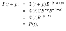
P(t) is periodic with period p. Solving equation (1.60) for ![]() , we get equation (1.59). □
, we get equation (1.59). □
Definition 1.106.
Let ![]() and C be as in Floquet’s theorem (Theorem 1.105). Then the eigenvalues μ of the matrix C are called the Floquet multipliers of the Floquet system (1.55).
and C be as in Floquet’s theorem (Theorem 1.105). Then the eigenvalues μ of the matrix C are called the Floquet multipliers of the Floquet system (1.55).
Since fundamental matrices of a linear system are not unique (see Theorem 1.85), we must show that the Floquet multipliers are well defined. Let ![]() and
and ![]() be fundamental matrices for the Floquet system (1.55) and let
be fundamental matrices for the Floquet system (1.55) and let
![]()
It remains to show that C 1 and C 2 have the same eigenvalues. By Theorem 1.85 there is a nonsingular constant matrix F so that
![]()
Hence,
![$$\displaystyle\begin{array}{rcl} C_{2}& =& \Psi ^{-1}(\alpha )\Psi (\alpha +p) {}\\ & =& [\Phi (\alpha )F]^{-1}[\Phi (\alpha +p)F] {}\\ & =& F^{-1}\Phi ^{-1}(\alpha )\Phi (\alpha +p)F {}\\ & =& F^{-1}C_{ 1}F. {}\\ \end{array}$$](fractional.files/image806.png)
Since
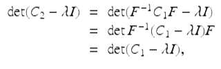
C 1 and C 2 have the same characteristic polynomial and therefore have the same eigenvalues. Hence Floquet multipliers are well defined.
Theorem 1.107.
The Floquet multipliers of the Floquet system (1.55) are the eigenvalues of the matrix
![]()
Proof.
To see this let ![]() be the fundamental matrix of the Floquet system (1.55) satisfying
be the fundamental matrix of the Floquet system (1.55) satisfying ![]() . Then the Floquet multipliers are the eigenvalues of
. Then the Floquet multipliers are the eigenvalues of
![]()
Iterating the equation
![]()
we get that
![$$\displaystyle\begin{array}{rcl} D& =& \Phi (\alpha +p) = [A(\alpha +p - 1)A(\alpha +p - 2)\cdots A(\alpha )]\Phi (\alpha ) {}\\ & =& A(\alpha +p - 1)A(\alpha +p - 2)\cdots A(\alpha ), {}\\ \end{array}$$](fractional.files/image812.png)
which is the desired result. □
Here are some simple examples of Floquet multipliers. Note that in the scalar case we use d instead of D.
Example 1.108.
For the scalar equation
![]()
the coefficient function a(t) = (−1) t has prime period p = 2, and d = a(1) a(0) = −1, so μ = −1 is the Floquet multiplier.
Example 1.109.
Find the Floquet multipliers for the Floquet system
![$$\displaystyle{u(t+1)\ = \left [\begin{array}{*{10}c} 0 &1\\ (-1)^{t } &0 \end{array} \right ]u(t),\quad t \in \mathbb{Z}_{0}.}$$](fractional.files/image814.png)
The coefficient matrix A(t) is periodic with prime period p = 2, so
![$$\displaystyle\begin{array}{rcl} D& =& \ A(1)A(0) {}\\ & =& \left [\begin{array}{ll} \;\;0 &1\\ - 1 &0 \end{array} \right ]\left [\begin{array}{ll} 0&1\\ 1 &0 \end{array} \right ] {}\\ & =& \left [\begin{array}{ll} 1&\;\;0\\ 0 & - 1 \end{array} \right ]. {}\\ \end{array}$$](fractional.files/image815.png)
Consequently, μ 1 = 1, μ 2 = −1 are the Floquet multipliers.
The following theorem demonstrates why the term multiplier is appropriate.
Theorem 1.110.
The number μ is a Floquet multiplier for the Floquet system (1.55) , if and only if there is a nontrivial solution u(t) of (1.55) such that
![]()
Furthermore, if μ 1 ,μ 2 ,⋯ ,μ k are distinct Floquet multipliers, then there are k linearly independent solutions, u i (t),1 ≤ i ≤ k of the Floquet system (1.55) on ![]() satisfying
satisfying
![]()
Proof.
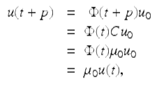
Assume μ 0 is a Floquet multiplier of (1.55). Then μ 0 is an eigenvalue of the matrix C given by equation (1.58). Let u 0 be an eigenvector of C corresponding to μ 0, and ![]() be a fundamental matrix for (1.55). Define
be a fundamental matrix for (1.55). Define
![]()
Then u(t) is a nontrivial solution of (1.55), and from Floquet’s theorem ![]() . Hence, we have
. Hence, we have
for ![]() The proof of the converse is essentially reversing the above steps. The proof of the last statement in this theorem is Exercise 1.89. □
The proof of the converse is essentially reversing the above steps. The proof of the last statement in this theorem is Exercise 1.89. □
In Example 1.109 we saw that 1 and − 1 were Floquet multipliers. Theorem 1.110 implies that there are linearly independent solutions that are periodic with periods 2 and 4. The next theorem shows how a Floquet system can be transformed into an autonomous system.
Theorem 1.111.
Let ![]() ,
, ![]() , be as in Floquet’s theorem. Then y(t) is a solution of the Floquet system (1.55) if and only if
, be as in Floquet’s theorem. Then y(t) is a solution of the Floquet system (1.55) if and only if
![]()
is a solution of the autonomous system
![]()
Proof.
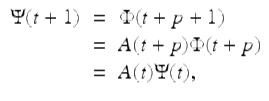
Assume y(t) is a solution of the Floquet system (1.55). Then there is a column vector w so that
![]()
Let z(t): = P −1(t)y(t), ![]() Then z(t) = P −1(t)y(t) = B t−α w. It follows that z(t) is a solution of z(t + 1) = Bz(t),
Then z(t) = P −1(t)y(t) = B t−α w. It follows that z(t) is a solution of z(t + 1) = Bz(t), ![]() The converse can be proved by reversing the above steps. □
The converse can be proved by reversing the above steps. □
Example 1.112.
In this example we determine the asymptotic behavior of two linearly independent solutions of the Floquet system
![$$\displaystyle{u(t+1)\ =\ \left [\begin{array}{ll} \;\;\;\;\;0 &\frac{2+(-1)^{t}} {2} \\ \frac{2-(-1)^{t}} {2} & \;\;\;\;\;0 \end{array} \right ]u(t),\quad t \in \mathbb{Z}_{0}.}$$](fractional.files/image827.png)
First we find the Floquet multipliers for this Floquet system. For this system, p = 2 and thus
![$$\displaystyle\begin{array}{rcl} D& =& A(1)A(0) {}\\ & =& \left [\begin{array}{ll} 0 &\frac{1} {2} \\ \frac{3} {2} & 0 \end{array} \right ]\left [\begin{array}{ll} 0 &\frac{3} {2} \\ \frac{1} {2} & 0 \end{array} \right ] {}\\ & =& \ \left [\begin{array}{ll} \frac{1} {4} & 0 \\ 0 &\frac{9} {4} \end{array} \right ]. {}\\ \end{array}$$](fractional.files/image828.png)
Hence the Floquet multipliers are ![]() and
and ![]() . Since
. Since ![]() and
and ![]() , we get there are two linearly independent solutions u 1(t), u 2(t) on
, we get there are two linearly independent solutions u 1(t), u 2(t) on ![]() satisfying
satisfying
![]()
Using Theorem 1.111 one can prove (see Exercise 1.92) the following stability theorem for Floquet systems.
Theorem 1.113.
Let μ 1 , μ 2 , ![]() , μ n be the Floquet multipliers of the Floquet system (1.55) . Then the trivial solution is
, μ n be the Floquet multipliers of the Floquet system (1.55) . Then the trivial solution is
(i)
globally asymptotically stable iff ![]() , 1 ≤ i ≤ n;
, 1 ≤ i ≤ n;
(ii)
stable provided ![]() 1 ≤ i ≤ n and whenever
1 ≤ i ≤ n and whenever ![]() , then μ i is a simple eigenvalue;
, then μ i is a simple eigenvalue;
(iii)
unstable provided there is an i 0 , 1 ≤ i 0 ≤ n, such that ![]()
Example 1.114.
By Theorem 1.113 the trivial solution of the Floquet system in Example 1.112 is globally asymptotically stable.
We conclude this section by mentioning that although in this chapter we have explored a substantial introduction to the classical difference calculus, there are naturally many stones we have left unturned. So, for the reader who is interested in more advanced and specialized techniques from the classical theory of difference equations, we encourage him or her to consult the book by Kelley and Peterson [135] for a multitude of related results.