Discrete Fractional Calculus (2015)
2. Discrete Delta Fractional Calculus and Laplace Transforms
2.2. The Delta Laplace Transform
In this section we develop properties of the (delta) Laplace transform. First we give an abstract definition of this transform.
Definition 2.1 (Bohner–Peterson [62]).
Assume ![]() Then we define the (delta) Laplace transform of f based at a by
Then we define the (delta) Laplace transform of f based at a by
for all complex numbers s ≠ − 1 such that this improper integral converges.
The following theorem gives two useful expressions for the Laplace transform of f.
Theorem 2.2.
Assume ![]() . Then
. Then
![]()
(2.1)
(2.2)
for all complex numbers s ≠ − 1 such that this improper integral (infinite series) converges.
Proof.
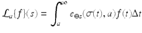
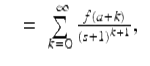
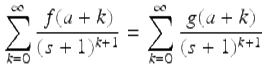
To see that (2.1) holds note that
![$$\displaystyle\begin{array}{rcl} \mathcal{L}_{a}\left \{f\right \}(s)& =& \int _{a}^{\infty }e_{ \ominus s}(\sigma (t),a)f(t)\Delta t {}\\ & =& \sum _{t=a}^{\infty }e_{ \ominus s}(\sigma (t),a)f(t) {}\\ & =& \sum _{t=a}^{\infty }[1 + \ominus s]^{\sigma (t)-a}f(t) {}\\ & =& \sum _{t=a}^{\infty } \frac{f(t)} {(1 + s)^{t-a+1}} {}\\ & =& \sum _{k=0}^{\infty } \frac{f(a + k)} {(1 + s)^{k+1}}. {}\\ \end{array}$$](fractional.files/image1016.png)
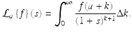
This also gives us that
□
To find functions such that the Laplace transform exists on a nonempty set we make the following definition.
Definition 2.3.
We say that a function ![]() is of exponential order r > 0 (at
is of exponential order r > 0 (at ![]() ) if there exists a constant A > 0 such that
) if there exists a constant A > 0 such that
![]()
Now we can prove the following existence theorem.
Theorem 2.4 (Existence Theorem).
Suppose ![]() is of exponential order r > 0. Then
is of exponential order r > 0. Then ![]() converges absolutely for |s + 1| > r.
converges absolutely for |s + 1| > r.
Proof.
Assume ![]() is of exponential order r > 0. Then there is a constant A > 0 and an
is of exponential order r > 0. Then there is a constant A > 0 and an ![]() such that for each
such that for each ![]()
![]() . Hence for | s + 1 | > r,
. Hence for | s + 1 | > r,
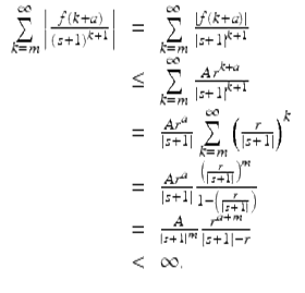
Hence, the Laplace transform of f converges absolutely for | s + 1 | > r. □
We will see later (see Remark 2.57) that the converse of Theorem 2.4 does not hold in general.
In this chapter, we will usually consider functions f of some exponential order r > 0, ensuring that the Laplace transform of f does in fact converge somewhere in the complex plane—specifically, it converges for all complex numbers outside the closed ball of radius r centered at negative one, that is, for | s + 1 | > r. We will abuse the notation by sometimes writing ![]() instead of the preferred notation
instead of the preferred notation ![]()
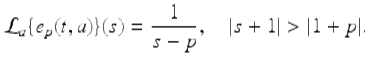
Example 2.5.
Clearly, ![]() p ≠ − 1, a constant, is of exponential order
p ≠ − 1, a constant, is of exponential order ![]() Therefore, we have for
Therefore, we have for ![]()
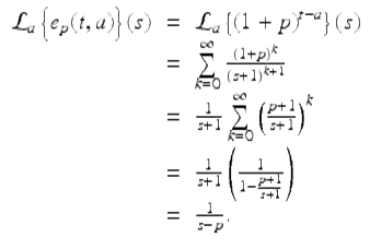
Hence
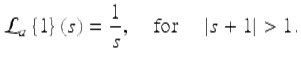
An important special case (p = 0) of the above formula is
In the next theorem we see that the Laplace transform operator ![]() is a linear operator.
is a linear operator.
Theorem 2.6 (Linearity).
Suppose ![]() and the Laplace transforms of f and g converge for |s + 1| > r, where r > 0, and let
and the Laplace transforms of f and g converge for |s + 1| > r, where r > 0, and let ![]() . Then the Laplace transform of c 1 f + c 2 g converges for |s + 1| > r and
. Then the Laplace transform of c 1 f + c 2 g converges for |s + 1| > r and
![]()
(2.3)
for |s + 1| > r.
Proof.
Since ![]() and the Laplace transforms of f and g converge for | s + 1 | > r, where r > 0, we have that for | s + 1 | > r
and the Laplace transforms of f and g converge for | s + 1 | > r, where r > 0, we have that for | s + 1 | > r
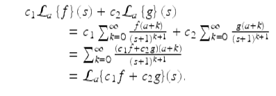
This completes the proof. □
The following uniqueness theorem is very useful.
Theorem 2.7 (Uniqueness).
Assume ![]() and there is an r > 0 such that
and there is an r > 0 such that
![]()
for |s + 1| > r. Then
![]()
Proof.
By hypothesis we have that
![]()
for | s + 1 | > r. This implies that
for | s + 1 | > r. It follows from this that
![]()
and this completes the proof. □
Next we give the Laplace transforms of the (delta) hyperbolic sine and cosine functions.
Theorem 2.8.
Assume p ≠ ± 1 is a constant. Then
(i)
![]()
(ii)
![]()
for ![]()
Proof.
To see that (ii) holds, consider
![$$\displaystyle\begin{array}{rcl} \mathcal{L}_{a}\{\sinh _{p}(t,a)\}(s)& =& \frac{1} {2}\left [\mathcal{L}_{a}\{e_{p}(t,a)\}(s) -\mathcal{L}\{e_{-p}(t,a)\}(s)\right ] {}\\ & =& \frac{1} {2} \frac{1} {s - p} -\frac{1} {2} \frac{1} {s + p} {}\\ & =& \frac{p} {s^{2} - p^{2}} {}\\ \end{array}$$](fractional.files/image1046.png)
for ![]() The proof of (i) is similar (see Exercise 2.5). □
The proof of (i) is similar (see Exercise 2.5). □
Next, we give the Laplace transforms of the (discrete) sine and cosine functions.
Theorem 2.9.
Assume p ≠ ± i. Then
(i)
![]()
(ii)
![]()
for ![]()
Proof.
To see that (i) holds, note that
![$$\displaystyle\begin{array}{rcl} \mathcal{L}_{a}\{\cos _{p}(t,a)\}(s)& =& \mathcal{L}_{a}\{\cosh _{ip}(t,a)\}(s) {}\\ & =& \frac{1} {2}\left [\mathcal{L}_{a}\{e_{ip}(t,a)\}(s) + \mathcal{L}\{e_{-ip}(t,a)\}(s)\right ] {}\\ & =& \frac{1} {2} \frac{1} {s - ip} + \frac{1} {2} \frac{1} {s + ip} {}\\ & =& \frac{s} {s^{2} + p^{2}}, {}\\ \end{array}$$](fractional.files/image1050.png)
for ![]() For the proof of part (ii) see Exercise 2.6. □
For the proof of part (ii) see Exercise 2.6. □
Theorem 2.10.
Assume α ≠ − 1 and ![]() Then
Then
(i)
![]()
(ii)
![]()
for ![]()
Proof.
To see that (i) holds, for ![]() consider
consider
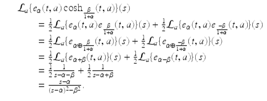
The proof of (ii) is Exercise 2.7. □
Similar to the proof of Theorem 2.10 one can prove the following theorem.
Theorem 2.11.
Assume α ≠ − 1 and ![]() Then
Then
(i)
![]()
(ii)
![]()
for ![]()
When solving certain difference equations one frequently uses the following theorem.
Theorem 2.12.
Assume that f is of exponential order r > 0. Then for any positive integer N
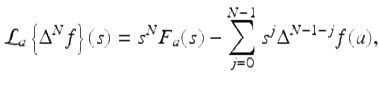
(2.4)
for |s + 1| > r.
Proof.
By Exercise 2.2 we have for each positive integer N, the function ![]() is of exponential order r. Hence, by Theorem 2.4 the Laplace transform of
is of exponential order r. Hence, by Theorem 2.4 the Laplace transform of ![]() for each N ≥ 1 exists for | s + 1 | > r. Now integrating by parts we get
for each N ≥ 1 exists for | s + 1 | > r. Now integrating by parts we get
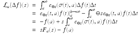
for | s + 1 | > r. Hence (2.4) holds for N = 1. Now assume N ≥ 1 and (2.4) holds. Then
![$$\displaystyle\begin{array}{rcl} \mathcal{L}_{a}\{\Delta ^{N+1}f\}(s)& =& \mathcal{L}_{ a}\{\Delta \left (\Delta ^{N}f\right )\}(s) {}\\ & =& s\mathcal{L}_{a}\{\Delta ^{N}f\}(s) - \Delta ^{N}f(a) {}\\ & =& s\left [s^{N}F_{ a}(s) -\sum \limits _{j=0}^{N-1}s^{j}\Delta ^{N-1-j}f(a)\right ] - \Delta ^{N}f(a) {}\\ & =& s^{N+1}F_{ a}(s) -\sum \limits _{j=0}^{(N+1)-1}s^{j}\Delta ^{(N+1)-1-j}f(a). {}\\ \end{array}$$](fractional.files/image1065.png)
Hence (2.4) holds for each positive integer by mathematical induction. □
The following example is an application of formula (2.4).
Example 2.13.
Use Laplace transforms to solve the IVP
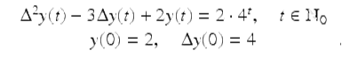
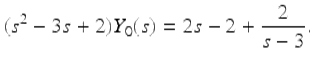
Assume y(t) is the solution of the above IVP. We have, by taking the Laplace transform of both sides of the difference equation in this example,
![$$\displaystyle{[s^{2}Y _{ 0}(s) - sy(0) - \Delta y(0)] - 3[sY _{0}(s) - y(0)] + 2Y _{0}(s) = \frac{2} {s - 3}.}$$](fractional.files/image1067.png)
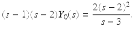
Applying the initial conditions and simplifying we get
Further simplification leads to
Hence
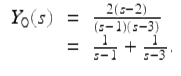
It follows that the solution of our IVP is given by
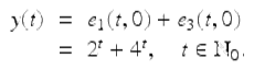
Now that we see that our solution is of exponential order we see that the steps we did above are valid.
The following corollary gives us a useful formula for solving certain summation (delta integral) equations.
Corollary 2.14.
Assume ![]() is of exponential order r > 1. Then
is of exponential order r > 1. Then
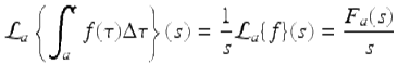
for |s + 1| > r.
Proof.
Since ![]() is of exponential order r > 1, we have by Exercise 2.3 that the function h defined by
is of exponential order r > 1, we have by Exercise 2.3 that the function h defined by
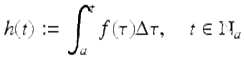
is also of exponential order r > 1. Hence the Laplace transform of h exists for | s + 1 | > r. Then
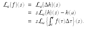
It follows that
for | s + 1 | > r. □
Example 2.15.
Solve the summation equation
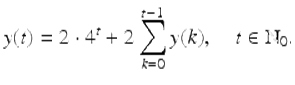
(2.5)
Equation (2.5) can be written in the equivalent form
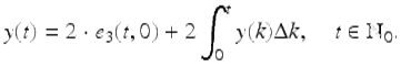
(2.6)
Taking the Laplace transform of both sides of (2.6) we get, using Corollary 2.14,
![]()
Solving for Y 0(s) we get
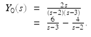
It follows that
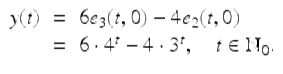
is the solution of (2.5).
Next we introduce the Dirac delta function and find its Laplace transform.
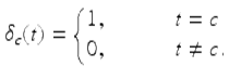
Definition 2.16.
Let ![]() . We define the Dirac delta function at c on
. We define the Dirac delta function at c on ![]() by
by
Theorem 2.17.
Assume ![]() . Then
. Then
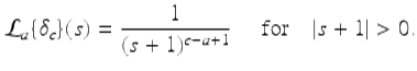
Proof.
For | s + 1 | > 0,
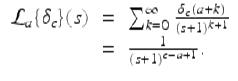
This completes the proof. □
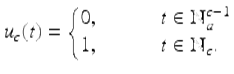
Next we define the unit step function and later find its Laplace transform.
Definition 2.18.
Let ![]() . We define the unit step function on
. We define the unit step function on ![]() by
by
We now prove the following shifting theorem.
Theorem 2.19 (Shifting Theorem).
Let ![]() and assume the Laplace transform of
and assume the Laplace transform of ![]() exists for |s + 1| > r. Then the following hold:
exists for |s + 1| > r. Then the following hold:
(i)
![]()
(ii)
![]()
for |s + 1| > r. (In (i) we have the convention that ![]() for
for ![]() if c ≥ a + 1.)
if c ≥ a + 1.)
Proof.
To see that (i) holds, consider
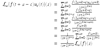
for | s + 1 | > r.
Part (ii) holds since
![$$\displaystyle\begin{array}{rcl} \mathcal{L}_{a}\{f(t + (c - a))\}(s)& =& \sum _{k=0}^{\infty }\frac{f(a + k + c - a)} {(s + 1)^{k+1}} {}\\ & =& \sum _{k=0}^{\infty } \frac{f(k + c)} {(s + 1)^{k+1}} {}\\ & =& \sum _{k=c-a}^{\infty } \frac{f(a + k)} {(s + 1)^{k-c+a+1}} {}\\ & =& (s + 1)^{c-a}\sum _{ k=c-a}^{\infty } \frac{f(a + k)} {(s + 1)^{k+1}} {}\\ & =& (s + 1)^{c-a}\left [\sum _{ k=0}^{\infty } \frac{f(a + k)} {(s + 1)^{k+1}} -\sum _{k=0}^{c-a-1} \frac{f(a + k)} {(s + 1)^{k+1}}\right ] {}\\ & =& (s + 1)^{c-a}\left [\mathcal{L}_{ a}\{f\}(s) -\sum _{k=0}^{c-a-1} \frac{f(a + k)} {(s + 1)^{k+1}}\right ] {}\\ \end{array}$$](fractional.files/image1090.png)
for | s + 1 | > r. □
In the following example we will use part (i) of Theorem 2.19 to solve an IVP.
Example 2.20.
Solve the IVP
Taking the Laplace transform of both sides, we get
Using the initial condition and solving for Y 0(s) we have that
Taking the inverse transform of both sides we get the desired solution
In the following example we will use part (ii) of Theorem 2.19 to solve an IVP.
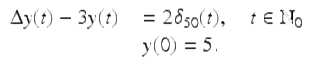
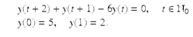
Example 2.21.
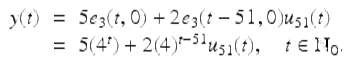
Use Laplace transforms to solve the IVP
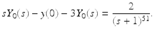
Assume y(t) is the solution of this IVP and take the Laplace transform of both sides of the given difference equation to get (using part (ii) of Theorem 2.19) that
![$$\displaystyle{(s + 1)^{2}\left [Y _{ 0}(s) - \frac{5} {s + 1} - \frac{2} {(s + 1)^{2}}\right ] + (s + 1)\left [Y _{0}(s) - \frac{5} {s + 1}\right ] - 6Y _{0}(s) = 0.}$$](fractional.files/image1096.png)
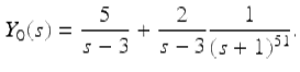
Solving for Y 0(s) we get
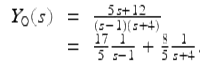
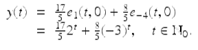
Taking the inverse transform of both sides we get
Theorem 2.22.
The following hold for n ≥ 0:
(i)
![]() for |s + 1| > 1;
for |s + 1| > 1;
(ii)
![]() for |s + 1| > 1.
for |s + 1| > 1.
Proof.
The proof of this theorem follows from Corollary 2.14 and the fact that ![]() for | s + 1 | > 1. □
for | s + 1 | > 1. □