Discrete Fractional Calculus (2015)
2. Discrete Delta Fractional Calculus and Laplace Transforms
2.3. Fractional Sums and Differences
The following theorem will motivate the definition of the n-th integer sum, which will in turn motivate the definition of the ν-th fractional sum. We will then define the ν-th fractional difference in terms of the ν-th fractional sum.
Theorem 2.23 (Repeated Summation Rule).
Let ![]() be given, then
be given, then
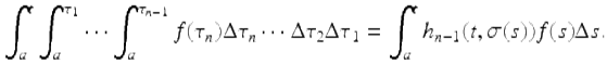
(2.7)
Proof.
We will prove this by induction on n for n ≥ 1. The case n = 1 is trivially true. Assume (2.7) holds for some n ≥ 1. It remains to show that (2.7) then holds when n is replaced by n + 1. To this end, let
![]()
Let ![]() , then it follows from the induction assumption that
, then it follows from the induction assumption that
where
![]()
It follows (using Theorem 1.61, (v)) that
![]()
Hence, integrating by parts, it follows that
This completes the proof. □
Motivated by (2.7), we define the n-th integer sum ![]() for positive integers n, by
for positive integers n, by
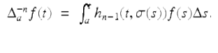
But, since
![]()
we obtain
![]()
(2.8)
which we consider the correct form of the n-th integer sum of f(t). Before we use the definition (2.8) of the n-th integer sum to motivate the definition of the ν-th fractional sum, we define the ν-th fractional Taylor monomial as follows.
Definition 2.24.
The ν-th fractional Taylor monomial based at s is defined by
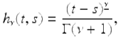
whenever the right-hand side is well defined.
We can now define the ν-th fractional sum.
Definition 2.25.
Assume ![]() and ν > 0. Then the ν-th fractional sum of f (based at a) is defined by
and ν > 0. Then the ν-th fractional sum of f (based at a) is defined by
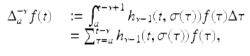
for ![]() Note that by our convention on delta integrals (sums) we can extend the domain of
Note that by our convention on delta integrals (sums) we can extend the domain of ![]() to
to ![]() , where N is the unique positive integer satisfying N − 1 < ν ≤ N, by noting that
, where N is the unique positive integer satisfying N − 1 < ν ≤ N, by noting that
![]()
The expression “fractional sum” is actually is misnomer as we define the ν-th fractional sum of a function for any ν > 0. Expressions like ![]() and
and ![]() are well defined.
are well defined.
Remark 2.26.
Note that the value of the ν-th fractional sum of f based at a is a linear combination of ![]() where the coefficient of f(t −ν) is one. In particular one can check that
where the coefficient of f(t −ν) is one. In particular one can check that ![]() has the form
has the form
![]()
(2.9)
The following formulas concerning the fractional Taylor monomials generalize the integer version of this theorem (Theorem 1.61).
Theorem 2.27.
Let ![]() . Then
. Then
(i)
h ν (t,t) = 0
(ii)
![]()
(iii)
![]()
(iv)
![]()
(v)
![]()
whenever these expressions make sense.
Proof.
To see that (iii) holds, note that
![$$\displaystyle\begin{array}{rcl} \Delta _{s}h_{\nu }(t,s)& =& h_{\nu }(t,s + 1) - h_{\nu }(t,s) {}\\ & =& \frac{(t - s - 1)^{\underline{\nu }}} {\Gamma (\nu +1)} -\frac{(t - s)^{\underline{\nu }}} {\Gamma (\nu +1)} {}\\ & =& \frac{\Gamma (t - s)} {\Gamma (t - s-\nu )\Gamma (\nu +1)} - \frac{\Gamma (t - s + 1)} {\Gamma (t - s + 1-\nu )\Gamma (\nu +1)} {}\\ & =& \bigg[(t - s-\nu ) - (t - s)\bigg] \frac{\Gamma (t - s)} {\Gamma (\nu +1)\Gamma (t - s -\nu +1)} {}\\ & =& - \frac{(\nu +1)\Gamma (t - s)} {\Gamma (\nu )\Gamma (t - s -\nu +1)} {}\\ & =& - \frac{\Gamma (t - s)} {\Gamma (\nu )\Gamma (t - s -\nu +1)} {}\\ & =& -\frac{(t -\sigma (s))^{\underline{\nu -1}}} {\Gamma (\nu )} {}\\ & =& -h_{\nu -1}(t,\sigma (s)). {}\\ \end{array}$$](fractional.files/image1129.png)
The rest of the proof of this theorem is Exercise 2.16. □
Example 2.28.
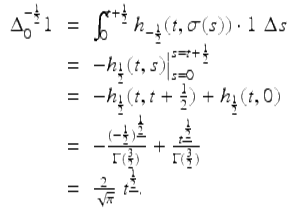
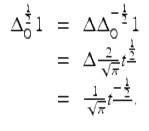
Using the definition of the fractional sum (Definition 2.25), find ![]()
Using Theorem 2.27, part (v), we get
Later we will give a formula (2.16) that also gives us this result.
Next we define the fractional difference in terms of the fractional sum.
Definition 2.29.
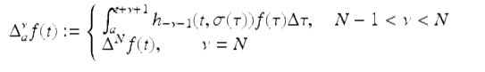
Assume ![]() and ν > 0. Choose a positive integer N such that N − 1 < ν ≤ N. Then we define the ν-th fractional difference by
and ν > 0. Choose a positive integer N such that N − 1 < ν ≤ N. Then we define the ν-th fractional difference by
![]()
Note that our fractional difference agrees with our prior understanding of whole-order differences—that is, for any ![]()
![]()
(2.10)
for ![]() . This is called the Riemann–Liouville definition of the ν-th delta fractional difference.
. This is called the Riemann–Liouville definition of the ν-th delta fractional difference.
Remark 2.30.
We will see in the proof of Theorem 2.35 below that the value of the fractional difference ![]() depends on the values of f on
depends on the values of f on ![]() . This full history nature of the value of the ν-th fractional difference of f is one of the important features of this fractional difference. In contrast if one is studying an n-th order difference equation, the term
. This full history nature of the value of the ν-th fractional difference of f is one of the important features of this fractional difference. In contrast if one is studying an n-th order difference equation, the term ![]() only depends on the values of f at the n + 1 points
only depends on the values of f at the n + 1 points ![]() .
.
Example 2.31.
Use Definition 2.29 to find ![]() Using Example 2.28, we have that
Using Example 2.28, we have that
Later we will give a formula (see (2.22)) that also gives us this result.
The following Leibniz formulas will be very useful.
Lemma 2.32 (Leibniz Formulas).
Assume ![]() . Then
. Then
![$$\displaystyle\begin{array}{rcl} \Delta \bigg[\int _{a}^{t-\mu +1}f(t,\tau )\Delta \tau \bigg] =\int _{ a}^{t-\mu +1}\Delta _{ t}f(t,\tau )\Delta \tau + f(t + 1,t -\mu +1)& &{}\end{array}$$](fractional.files/image1144.png)
(2.11)
and
![$$\displaystyle\begin{array}{rcl} \Delta \bigg[\int _{a}^{t-\mu +1}f(t,\tau )\Delta \tau \bigg] =\int _{ a}^{t-\mu +2}\Delta _{ t}f(t,\tau )\Delta \tau + f(t,t -\mu +1)& &{}\end{array}$$](fractional.files/image1145.png)
(2.12)
for ![]() where the
where the ![]() inside the integral means the difference of f(t,τ) with respect to t.
inside the integral means the difference of f(t,τ) with respect to t.
Proof.
To see that (2.11) holds, note that, for ![]() ,
,
![$$\displaystyle\begin{array}{rcl} \Delta \bigg[\int _{a}^{t-\mu +1}f(t,\tau )\Delta \tau \bigg]& =& \int _{ a}^{t-\mu +2}f(t + 1,\tau )\Delta \tau -\int _{ a}^{t-\mu +1}f(t,\tau )\Delta \tau {}\\ & =& \int _{a}^{t-\mu +1}\Delta _{ t}f(t,\tau )\Delta \tau + f(t + 1,t + 1-\mu ). {}\\ \end{array}$$](fractional.files/image1149.png)
The proof of (2.12) is Exercise 2.19. □
In the next theorem we give a very useful formula for ![]() . We call this formula the alternate definition of
. We call this formula the alternate definition of ![]() (see Holm [123, 124]).
(see Holm [123, 124]).
Theorem 2.33.
Let ![]() and ν > 0 be given, with N − 1 < ν ≤ N. Then
and ν > 0 be given, with N − 1 < ν ≤ N. Then
(2.13)
for ![]()
Proof.
First note that if ![]() then using (2.10), we have that
then using (2.10), we have that
![]()
Now assume N − 1 < ν < N. Our proof of (2.13) will follow from N applications of the Leibniz formula (2.12). To see this we have for ![]()
![$$\displaystyle\begin{array}{rcl} \Delta _{a}^{\nu }f(t)& =& \Delta ^{N}\Delta _{ a}^{-\left (N-\nu \right )}f(t) {}\\ & =& \Delta ^{N}\left [\int _{ a}^{t-(N-\nu )+1}h_{ N-\nu -1}(t,\sigma (\tau ))f(\tau )\Delta \tau \right ] {}\\ & =& \Delta ^{N-1} \cdot \Delta \bigg[\int _{ a}^{t-(N-\nu )+1}h_{ N-\nu -1}(t,\sigma (\tau ))f(\tau )\Delta \tau \bigg]. {}\\ \end{array}$$](fractional.files/image1157.png)
Using the Leibniz rule (2.12), we get
![$$\displaystyle\begin{array}{rcl} \Delta _{a}^{\nu }f(t)& & = \Delta ^{N-1}\Bigg[\int _{ a}^{t-(N-\nu -1)+1}h_{ N-\nu -2}(t,\sigma (\tau ))f(\tau )\Delta \tau {}\\ & & \quad \quad \quad \quad + h_{N-\nu -1}(t,t - (N -\nu -2))f(t - (N -\nu -1))\Bigg] {}\\ & & = \Delta ^{N-1}\left [\int _{ a}^{t-(N-\nu -1)+1}h_{ N-\nu -2}(t,\sigma (\tau ))f(\tau )\Delta \tau \right ]. {}\\ & & {}\\ \end{array}$$](fractional.files/image1158.png)
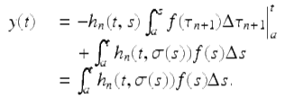
Applying the Leibniz formula (2.12) again we get
![$$\displaystyle\begin{array}{rcl} \Delta _{a}^{\nu }f(t)& & = \Delta ^{N-2}\Bigg[\int _{ a}^{t-(N-\nu -2)+1}h_{ N-\nu -3}(t,\sigma (\tau ))f(\tau )\Delta \tau {}\\ & & \quad \quad \quad \quad + h_{N-\nu -2}(t,t - (N -\nu -3))f(t - (N -\nu -2))\Bigg] {}\\ & & = \Delta ^{N-2}\left [\int _{ a}^{t-(N-\nu -2)+1}h_{ N-\nu -3}(t,\sigma (\tau ))f(\tau )\Delta \tau \right ]. {}\\ & & {}\\ \end{array}$$](fractional.files/image1159.png)
Repeating these steps N − 2 more times, we find that
![$$\displaystyle\begin{array}{rcl} \Delta _{a}^{\nu }f(t)& & = \Delta ^{N-N}\Bigg[\int _{ a}^{t-(N-\nu -N)+1}h_{ N-\nu -N-1}(t,\sigma (\tau ))f(\tau )\Delta \tau {}\\ & & \quad \quad + h_{N-\nu -N}(t,t - (N -\nu -(N + 1))f(t - (N -\nu -N))\Bigg] {}\\ & & =\int _{ a}^{t+\nu +1}h_{ -\nu -1}(t,\sigma (\tau ))f(\tau )\Delta \tau + h_{-\nu }(t,t +\nu +1)f(t+\nu ) {}\\ & & =\int _{ a}^{t+\nu +1}h_{ -\nu -1}(t,\sigma (\tau ))f(\tau )\Delta \tau. {}\\ \end{array}$$](fractional.files/image1160.png)
This completes the proof. □
Remark 2.34.
By Theorem 2.33 we get for all ν > 0, ![]() that the formula for
that the formula for ![]() can be obtained from the formula for
can be obtained from the formula for ![]() in Definition 2.25 by replacing ν by −ν and vice-versa, but the domains are different.
in Definition 2.25 by replacing ν by −ν and vice-versa, but the domains are different.
Theorem 2.35 (Existence-Uniqueness Theorem).
Assume ![]() , ν > 0 and N is a positive integer such that N − 1 < ν ≤ N. Then the initial value problem
, ν > 0 and N is a positive integer such that N − 1 < ν ≤ N. Then the initial value problem
![]()
(2.14)
![]()
(2.15)
where A i , 0 ≤ i ≤ N − 1, are given constants, has a unique solution on ![]()
Proof.
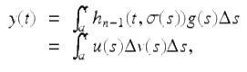
Note that by Remark 2.26, for each fixed t, ![]() is a linear combination of
is a linear combination of ![]() with the coefficient of
with the coefficient of ![]() being one. Since
being one. Since
![]()
we have for each fixed t, ![]() is a linear combination of
is a linear combination of ![]() , ⋯ , y(t +ν), where the coefficient of y(t +ν) is one. Now define y(t) on
, ⋯ , y(t +ν), where the coefficient of y(t +ν) is one. Now define y(t) on ![]() by the initial conditions (2.15). Then note that y(t) satisfies the fractional difference equation (2.14) at t = 0 iff
by the initial conditions (2.15). Then note that y(t) satisfies the fractional difference equation (2.14) at t = 0 iff
![]()
But this holds iff
![]()
which is equivalent to the equation
![]()
Hence if we define y(ν) to be the solution of this last equation, then y(t) satisfies the fractional difference equation at t = 0. Summarizing, we have shown that knowing y(t) at the points ![]() , 0 ≤ i ≤ N − 1 uniquely determines what the value of the solution is at the next point ν. Next one uses the fact that the values of y(t) on
, 0 ≤ i ≤ N − 1 uniquely determines what the value of the solution is at the next point ν. Next one uses the fact that the values of y(t) on ![]() uniquely determine the value of the solution at ν + 1. An induction argument shows that the solution is uniquely determined on
uniquely determine the value of the solution at ν + 1. An induction argument shows that the solution is uniquely determined on ![]() □
□
Remark 2.36.
We could easily extend Theorem 2.35 to the case when ![]() instead of the special case a = 0 that we considered in Theorem 2.35. Also, the term
instead of the special case a = 0 that we considered in Theorem 2.35. Also, the term ![]() in equation (2.14) could be replaced by
in equation (2.14) could be replaced by ![]() for any 0 ≤ i ≤ N − 1. Note that we picked the nice set
for any 0 ≤ i ≤ N − 1. Note that we picked the nice set ![]() so that the fractional difference equation needs to be satisfied for all
so that the fractional difference equation needs to be satisfied for all ![]() , but then solutions are defined on the shifted set
, but then solutions are defined on the shifted set ![]() By shifting the set on which the fractional difference equation is defined, we can evidently obtain solutions that are defined on the nicer set
By shifting the set on which the fractional difference equation is defined, we can evidently obtain solutions that are defined on the nicer set ![]() . In this book our convention when considering fractional difference equations is to assume the fractional difference equation is satisfied for
. In this book our convention when considering fractional difference equations is to assume the fractional difference equation is satisfied for ![]() and the solutions are defined on
and the solutions are defined on ![]()
In a standard manner one gets the following result that follows from Theorem 2.35.
Theorem 2.37.
Assume ![]() . Then the homogeneous fractional difference equation
. Then the homogeneous fractional difference equation
![]()
has N linearly independent solutions u i (t), 1 ≤ i ≤ N, on ![]() and
and
![]()
where c 1 ,c 2 ,⋯ ,c N are arbitrary constants, is a general solution of this homogeneous fractional difference equation on ![]() . Furthermore, if in addition, y p (t) is a particular solution of the nonhomogeneous fractional difference equation ( 2.14) on
. Furthermore, if in addition, y p (t) is a particular solution of the nonhomogeneous fractional difference equation ( 2.14) on ![]() , then
, then
![]()
where c 1 ,c 2 ,⋯ ,c N are arbitrary constants, is a general solution of the nonhomogeneous fractional difference equation ( 2.14).