Discrete Fractional Calculus (2015)
2. Discrete Delta Fractional Calculus and Laplace Transforms
2.4. Fractional Power Rules
Using the Leibniz formula we will prove the following fractional sum power rule. Later in this chapter (see Theorem 2.72) we will use discrete Laplace transforms to give an easier proof of this theorem. Later we will see that the fractional difference power rule (Theorem 2.40) will follow from this fractional sum power rule.
Theorem 2.38 (Fractional Sum Power Rule).
Assume μ ≥ 0 and ν > 0. Then
![]()
(2.16)
for ![]()
Proof.
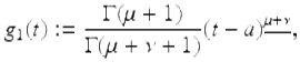
Let
and
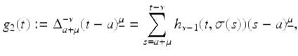
(2.17)
for ![]() To complete the proof we will show that both of these functions satisfy the initial value problem
To complete the proof we will show that both of these functions satisfy the initial value problem
![]()
(2.18)
![]()
(2.19)
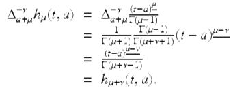
Since
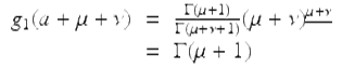
and
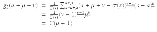
we have that g i (t), i = 1, 2 both satisfy the initial condition (2.19).
We next show that g 1(t) satisfies the difference equation (2.18). Note that
![]()
Multiplying both sides by ![]() we obtain
we obtain
^{\underline{\mu +\nu -1}} {}\\ & =& (\mu +\nu ) \frac{\Gamma (\mu +1)} {\Gamma (\mu +\nu + 1)}(t - a)^{\underline{\mu +\nu }}\quad \quad \mbox{ by Exercise (1.9)} {}\\ & =& (\mu +\nu )g_{1}(t) {}\\ \end{array}$$](fractional.files/image1200.png)
for ![]() That is, g 1(t) is a solution of (2.18).
That is, g 1(t) is a solution of (2.18).
It remains to show that g 2(t) satisfies (2.18). Using (2.17) we have that
)^{\underline{\nu -2}}(s - a)^{\underline{\mu }} {}\\ & & = \frac{1} {\Gamma (\nu )}\sum _{s=a+\mu }^{t-\nu }\big[(t - a - (\mu +\nu ) + 1) - (s - a-\mu )\big](t -\sigma (s))^{\underline{\nu -2}}(s - a)^{\underline{\mu }} {}\\ & & = \frac{t - a - (\mu +\nu ) + 1} {\Gamma (\nu )} \sum _{s=a+\mu }^{t-\nu }(t -\sigma (s))^{\underline{\nu -2}}(s - a)^{\underline{\mu }} {}\\ & & - \frac{1} {\Gamma (\nu )}\sum _{s=a+\mu }^{t-\nu }(t -\sigma (s))^{\underline{\nu -2}}(s - a-\mu )(s - a)^{\underline{\mu }} {}\\ & & = h(t) - k(t), {}\\ \end{array}$$](fractional.files/image1201.png)
where
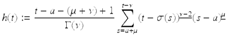
and

Using (2.17) and (2.11) we get
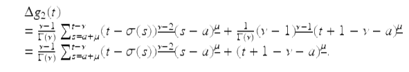
It follows that
![]()
(2.20)
Also, integrating by parts we get (here we also use Lemma 2.32)
![$$\displaystyle\begin{array}{rcl} k(t)& =& \frac{1} {\Gamma (\nu )}\sum _{s=a+\mu }^{t-\nu }(t -\sigma (s))^{\underline{\nu -2}}(s - a)^{\underline{\mu +1}} {}\\ & =& \frac{1} {\Gamma (\nu )}\left [-\frac{(s - a)^{\underline{\mu +1}}(t - s)^{\underline{\nu -1}}} {\nu -1} \right ]_{s=a+\mu }^{s=t+1-\nu } {}\\ & & + \frac{\mu +1} {(\nu -1)\Gamma (\nu )}\sum _{s=a+\mu }^{t-\nu }(t -\sigma (s))^{\underline{\nu -1}}(s - a)^{\underline{\mu }} {}\\ & =& -\frac{(t + 1 -\nu -a)^{\underline{\mu +1}}} {\nu -1} + \frac{\mu +1} {(\nu -1)\Gamma (\nu )}\sum _{s=a+\mu }^{t-\nu }(t -\sigma (s))^{\underline{\nu -1}}(s - a)^{\underline{\mu }}. {}\\ \end{array}$$](fractional.files/image1206.png)
It follows that
![]()
(2.21)
Finally, from (2.21) and (2.20), we get
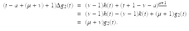
This completes the proof. □
Example 2.39.
Find
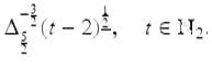
Consider
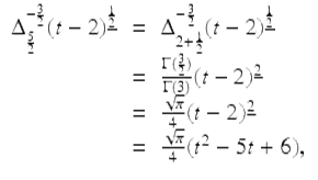
for ![]()
Theorem 2.40 (Fractional Difference Power Rule).
Assume μ > 0 and ν ≥ 0, N − 1 < ν < N. Then
![]()
(2.22)
for ![]()
Proof.
To see that (2.22) holds, note that
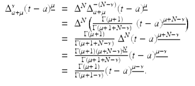
This completes the proof. □
Example 2.41.
Find

Consider
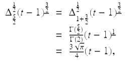
for ![]()
The fractional power rules in terms of Taylor monomials take a nice form as we see in the following theorem.
Theorem 2.42.
Assume μ > 0, ν > 0, then the following hold:
(i)
![]()
(ii)
![]()
Proof.
To see that (i) follows from Theorem 2.38 note that for ![]()
Similarly, part (ii) follows from Theorem 2.40 (see Exercise 2.22). □
Theorem 2.43.
Assume μ > 0 and N is a positive integer such that N − 1 < μ ≤ N. Then for any constant a
![]()
for all constants c 1 ,c 2 ,⋯ ,c N , is a solution of the fractional difference equation ![]() on
on ![]()
Proof.
Let μ and N be as in the statement of this theorem. If μ = N, then for 1 ≤ k ≤ N, we have that
![]()
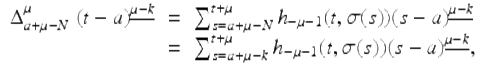
Now assume that N − 1 < μ < N. Then we want to consider the expression
![]()
Note that since the subscript and the exponent do not match up in the correct way we cannot immediately apply formula (2.22) to the above expression. To compensate for this we do the following.
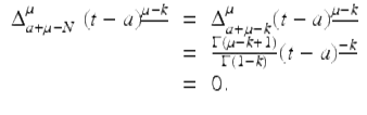
since
![]()
Therefore, we have that
The conclusion of the theorem then follows from the fact that ![]() is a linear operator. □
is a linear operator. □
It follows from Theorem 2.43 that
![]()
is a general solution of ![]()
Theorem 2.44 (Continuity of Fractional Differences).
Let ![]() be given. Then the fractional difference
be given. Then the fractional difference ![]() is continuous with respect to ν for ν > 0. By this we mean for each fixed
is continuous with respect to ν for ν > 0. By this we mean for each fixed ![]() ,
,
![]()
where ⌈ν⌉ denotes the ceiling of ν, is continuous for ν > 0.
Proof.
To prove this theorem it suffices to prove the following:
(i)
![]() is continuous with respect to ν on (N − 1, N);
is continuous with respect to ν on (N − 1, N);
(ii)
![]()
(iii)
![]()
First we show that (i) holds. For any fixed ν > 0 with N − 1 < ν < N, we have
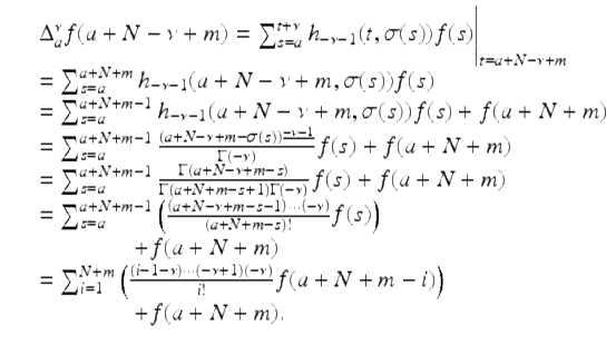
It follows from this last expression that ![]() is a continuous function of ν, for N − 1 < ν < N.
is a continuous function of ν, for N − 1 < ν < N.
![$$\displaystyle\begin{array}{rcl} & & \lim _{\nu \rightarrow N^{-}}\Delta _{a}^{\nu }f(a + N -\nu +m) {}\\ & & =\lim _{\nu \rightarrow N^{-}}\Big[\sum _{i=1}^{N+m}\left (\frac{\left (i - 1-\nu \right ) \cdot \cdot \cdot \left (-\nu \right )} {i!} f(a + N + m - i)\right ) {}\\ & & \quad \quad \quad \quad + f(a + N + m)\Big] {}\\ & & =\sum _{ i=1}^{N+m}\left (\frac{\left (i - 1 - N\right ) \cdot \cdot \cdot \left (-N\right )} {i!} f(a + N + m - i)\right ) + f(a + N + m) {}\\ & & =\sum _{ i=1}^{N}\left (\frac{\left (i - 1 - N\right ) \cdot \cdot \cdot \left (-N\right )} {i!} f(a + N + m - i)\right ) + f(a + N + m), {}\\ & & =\sum _{ i=1}^{N}\left ((-1)^{i}\frac{(N) \cdot \cdot \cdot (N - i + 1)} {i!} f(a + N + m - i)\right ) + f(a + N + m) {}\\ & & =\sum _{ i=1}^{N}\left ((-1)^{i}\binom{N}{i}f(a + N + m - i)\right ) {}\\ & & \quad \quad \quad + f(a + N + m) {}\\ & & =\sum _{ i=0}^{N}(-1)^{i}\binom{N}{i}f(a + N + m - i) {}\\ & & =\sum _{ i=0}^{N}(-1)^{i}\binom{N}{i}f((a + m) + N - i) {}\\ & & = \Delta ^{N}f(a + m). {}\\ \end{array}$$](fractional.files/image1241.png)
Hence, (ii) holds.
Finally, we show (iii) holds. To see this consider
![$$\displaystyle\begin{array}{rcl} & & \lim _{\nu \rightarrow (N-1)^{+}}\Delta _{a}^{\nu }f(a + N -\nu +m) {}\\ & =& \lim _{\nu \rightarrow (N-1)^{+}}\Bigg[\sum _{i=1}^{N+m}\left (\frac{\left (i - 1-\nu \right ) \cdot \cdot \cdot \left (-\nu \right )} {i!} f(a + N + m - i)\right ) {}\\ & & \qquad \qquad \qquad \qquad \qquad \qquad + f(a + N + m)\Bigg] {}\\ & =& \sum _{i=1}^{N+m}\left (\frac{\left (i - N\right ) \cdot \cdot \cdot \left (-N + 1\right )} {i!} f(a + N + m - i)\right ) + f(a + N + m) {}\\ & =& \sum _{i=1}^{N-1}\left (\frac{\left (i - N\right ) \cdot \cdot \cdot \left (-N + 1\right )} {i!} f(a + N + m - i)\right ) + f(a + N + m) {}\\ & =& \sum _{i=1}^{N-1}\left ((-1)^{i}\frac{\left (N - 1\right ) \cdot \cdot \cdot \left (N - i\right )} {i!} f(a + N + m - i)\right ) {}\\ & \; & \quad \quad \quad \quad + f(a + N + m)\ \ \ {}\\ & =& \sum _{i=1}^{N-1}\left ((-1)^{i}\binom{N - 1}{i}f(a + N + m - i)\right ) + f(a + N + m) {}\\ \qquad & =& \sum _{i=0}^{N-1}\left ((-1)^{i}\binom{N - 1}{i}f(a + m + 1 + (N - 1) - i)\right ) {}\\ & =& \Delta ^{N-1}f(a + m + 1). {}\\ \end{array}$$](fractional.files/image1242.png)
Hence, (iii) holds. □
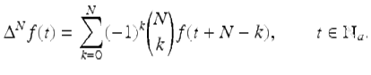
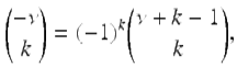
The binomial expression for ![]() is given by
is given by
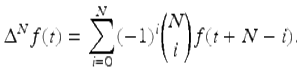
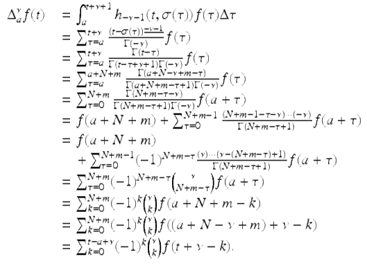
In the following theorem we give the binomial expressions for fractional differences and fractional sums.
Theorem 2.45 (Fractional Binomial Formulas).
Assume N − 1 < ν ≤ N and ![]() . Then
. Then
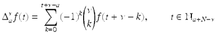
(2.23)
and
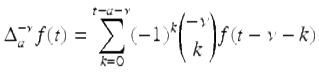
(2.24)
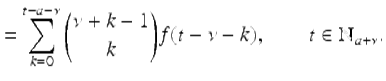
(2.25)
Proof.
Assume ![]() and 0 ≤ ν ≤ N. Fix
and 0 ≤ ν ≤ N. Fix ![]() . Then
. Then ![]() for some
for some ![]() Then
Then
Hence (2.23) holds. Since we can obtain the formula for ![]() from the formula for
from the formula for ![]() by replacing ν by −ν we get that (2.24) holds with the appropriate change in domains. Finally, since
by replacing ν by −ν we get that (2.24) holds with the appropriate change in domains. Finally, since
(2.25) follows immediately from (2.24). □
Note that if we let ν = N in (2.23), we get the following integer binomial expression for ![]() , that is
, that is