Discrete Fractional Calculus (2015)
2. Discrete Delta Fractional Calculus and Laplace Transforms
2.11. Exercises
2.1. Show that ![]() is of exponential order r = 1 iff f is bounded on
is of exponential order r = 1 iff f is bounded on ![]() .
.
2.2. Prove that if ![]() is of exponential order r > 0, then
is of exponential order r > 0, then ![]() is also of exponential order r for
is also of exponential order r for ![]()
2.3. Show that if ![]() is of exponential order r > 1, then
is of exponential order r > 1, then ![]()
![]() ,
, ![]() is also of exponential order r.
is also of exponential order r.
2.4. Show that h 0(t, a) is of exponential order 1 and for each n ≥ 0, h n (t, a) is of exponential order 1 +ε for all ε > 0.
2.5. Prove formula (i) in Theorem 2.8, that is
![]()
for ![]()
2.6. Prove formula (ii) in Theorem 2.9, that is
![]()
for ![]()
2.7. Prove formula (ii) in Theorem 2.10, that is
for ![]()
2.8. Prove Theorem 2.11.
2.9. For each of the following find y(t) given that
(i)
![]()
(ii)
![]()
2.10. Use Laplace transforms to solve the following IVPs
(i)

(ii)

(iii)

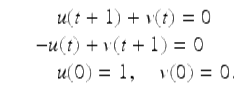
2.11. Use Laplace transforms to solve the IVP
2.12. Solve each of the following IVPs:
(i)

(ii)

2.13. Solve the following summation equations using Laplace transforms:
(i)
![]()
(ii)
![]()
(iii)
![]()
(iv)
![]()
2.14. Use Laplace transforms to solve each of the following:
(i)
![]()
(ii)
![]()
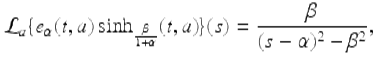
2.15. Show that
(i)
![]()
(ii)
![]()
2.16. Complete the proof of Theorem 2.27.
2.17. Work each of the following:
(i)
Use the definition of the ν-th fractional sum (Definition 2.25) to find ![]()
(ii)
Use the definition of the fractional difference (Definition 2.29) and part (2.32) to find ![]()
2.18. Show that the following hold:
(i)
![]()
(ii)
![]()
2.19. Verify that (2.12) holds.
2.20. Show that ![]() for
for ![]() ,
, ![]()
2.21. Evaluate each of the following using Theorem 2.38 and Theorem 2.40
(i)
![]()
(ii)
![]()
(iii)
![]()
(iv)

2.22. Prove that part (ii) of Theorem 2.42, follows from Theorem 2.40.
2.23. Prove (2.26).
2.24. Solve each of the following IVPs:
(i)
![]()
(ii)
![]()
(iii)
![]()
2.25. Use Theorems 2.54 and 2.58 to show that ![]() . Evaluate the convolution product 1 ∗ 1 and show directly (do not use the convolution theorem) that
. Evaluate the convolution product 1 ∗ 1 and show directly (do not use the convolution theorem) that ![]()
![]()
2.26. Assume ![]() and p ≠ 0. Using the definition of the convolution product (Definition 2.59), find
and p ≠ 0. Using the definition of the convolution product (Definition 2.59), find
![]()
2.27. Assume ![]() and p ≠ q. Using the definition of the convolution product (Definition 2.59), find
and p ≠ q. Using the definition of the convolution product (Definition 2.59), find
![]()
2.28. For N a positive integer, use the definition of the Laplace transform to prove that (2.4) holds (that is, (2.52) holds when ν = N).
Bibliography
3.
Ahrendt, K., Castle, L., Holm, M., Yochman, K.: Laplace transforms for the nabla-difference operator and a fractional variation of parameters formula. Commun. Appl. Anal. 16, 317–347 (2012)MathSciNetMATH
31.
Atici, F.M., Eloe, P.W.: Two-point boundary value problems for finite fractional difference equations. J. Differ. Equ. Appl. 17, 445–456 (2011)CrossRefMathSciNetMATH
32.
Atici, F.M., Eloe, P.W.: A transform method in discrete fractional calculus. Int. J. Differ. Equ. 2, 165–176 (2007)MathSciNet
34.
Atici, F.M., Eloe, P.W.: Initial value problems in discrete fractional calculus. Proc. Am. Math. Soc. 137, 981–989 (2009)CrossRefMathSciNetMATH
35.
Atici, F.M., Eloe, P.W.: Discrete fractional calculus with the nabla operator. Electron. J. Qual. Theory Differ. Equ., Spec. Ed. I 3, 1–12 (2009)
36.
Atici, F.M., Eloe, P.W.: Linear forward fractional difference equations. Commun. Appl. Anal. 19, 31–42 (2015)
62.
Bohner, M., Peterson, A.: Dynamic Equations on Time Scales: An Introduction with Application. Birkhäuser, Boston, MA (2001)CrossRef
88.
Goodrich, C.S.: Solutions to a discrete right-focal boundary value problem. Int. J. Differ. Equ. 5, 195–216 (2010)MathSciNet
89.
Goodrich, C.S.: Continuity of solutions to discrete fractional initial value problems. Comput. Math. Appl. 59, 3489–3499 (2010)CrossRefMathSciNetMATH
91.
Goodrich, C.S.: Some new existence results for fractional difference equations. Int. J. Dyn. Syst. Differ. Equ. 3, 145–162 (2011)MathSciNetMATH
92.
Goodrich, C.S.: Existence and uniqueness of solutions to a fractional difference equation with nonlocal conditions. Comput. Math. Appl. 61, 191–202 (2011)CrossRefMathSciNetMATH
94.
Goodrich, C.S.: Existence of a positive solution to a system of discrete fractional boundary value problems. Appl. Math. Comput. 217, 4740–4753 (2011)CrossRefMathSciNetMATH
95.
Goodrich, C.S.: Existence of a positive solution to a first-order p-Laplacian BVP on a time scale. Nonlinear Anal. 74, 1926–1936 (2011)CrossRefMathSciNetMATH
96.
Goodrich, C.S.: On positive solutions to nonlocal fractional and integer-order difference equations. Appl. Anal. Discrete Math. 5, 122–132 (2011)CrossRefMathSciNetMATH
123.
Holm, M.: Sum and difference compositions in discrete fractional calculus. Cubo 13, 153–184 (2011)CrossRefMathSciNetMATH
124.
Holm, M.: Solutions to a discrete, nonlinear, (N − 1, 1) fractional boundary value problem. Int. J. Dyn. Syst. Differ. Equ. 3, 267–287 (2011)MathSciNetMATH
125.
Holm, M.: The theory of discrete fractional calculus: development and application. PhD Dissertation, University of Nebraska-Lincoln (2011)
146.
Miller, K.S., Ross, B.: Fractional Difference Calculus. In: Proceedings of the International Symposium on Univalent Functions, Fractional Calculus and their Applications, Nihon University, Koriyama, Japan, 1988, 139–152; Ellis Horwood Ser. Math. Appl, Horwood, Chichester (1989)
147.
Miller, K.S., Ross, B.: An Introduction to the Fractional Calculus and Fractional Difference Equations. Wiley, New York (1993)
152.
Oldham, K., Spanier, J.: The Fractional Calculus: Theory and Applications of Differentiation and Integration to Arbitrary Order. Dover Publications, Mineola, New York (2002)
153.
Podlubny, I.: Fractional Differential Equations. Academic Press, New York (1999)MATH