Discrete Fractional Calculus (2015)
3. Nabla Fractional Calculus
3.3. Nabla Exponential Function
In this section we want to study the nabla exponential function that plays a similar role in the nabla calculus that the exponential function e pt does in the continuous calculus. Motivated by the fact that when p is a constant, x(t) = e ptis the unique solution of the initial value problem
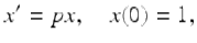
we define the nabla exponential function, E p (t, s) based at  , where the function p is in the set of (nabla) regressive functions

to be the unique solution of the initial value problem

(3.5)

(3.6)
After reading the proof of the next theorem one sees why this IVP has a unique solution. In the next theorem we give a formula for the exponential function E p (t, s).
Theorem 3.6.
Assume  and
and  . Then
![$$\displaystyle{ E_{p}(t,s) = \left \{\begin{array}{@{}l@{\quad }l@{}} \prod _{\tau =s+1}^{t} \frac{1} {1-p(\tau )}\text{, } \quad &t \in \mathbb{N}_{s} \\ \prod _{\tau =t+1}^{s}[1 - p(\tau )]\text{, }\quad &t \in \mathbb{N}_{a}^{s-1}. \end{array} \right. }$$](fractional.files/image1567.png)
(3.7)
Here it is understood that  for any function h.
Proof.
First we find a formula for E p (t, s) for t ≥ s + 1 by solving the IVP (3.5), (3.6) by iteration. Solving the nabla difference equation (3.5) for y(t) we obtain

(3.8)
Letting  in (3.8) we get

Then letting  in (3.8) we obtain
![$$\displaystyle{y(s + 2) = \frac{1} {1 - p(s + 2)}y(s + 1) = \frac{1} {\left [1 - p(s + 1)\right ]\left [1 - p(s + 2)\right ]}.}$$](fractional.files/image1573.png)
Proceeding in this matter we get by mathematical induction that
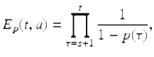
for  . By our convention on products we get
![$$\displaystyle{E_{p}(s,s) =\prod _{ \tau =s+1}^{s}[1 - p(\tau )] = 1}$$](fractional.files/image1576.png)
as desired. Now assume a ≤ t < s. Solving the nabla difference equation (3.5) for y(t − 1) we obtain
![$$\displaystyle\begin{array}{rcl} y(t - 1) = [1 - p(t)]y(t),\quad t \in \mathbb{N}_{a+1}.& &{}\end{array}$$](fractional.files/image1577.png)
(3.9)
Letting t = s in (3.9) we get
![$$\displaystyle{y(s - 1) = [1 - p(s)]y(s) = [1 - p(s)].}$$](fractional.files/image1578.png)
If s − 2 ≥ a, we obtain by letting  in (3.9)
![$$\displaystyle{y(s - 2) = [1 - p(s - 1)]y(s - 1) = \left [1 - p(s)\right ]\left [1 - p(s - 1)\right ].}$$](fractional.files/image1580.png)
By mathematical induction we arrive at
![$$\displaystyle{E_{p}(t,s) =\prod _{ \tau =t+1}^{s}[1 - p(\tau )],\quad \mbox{ for}\quad t \in \mathbb{N}_{ a}^{s}.}$$](fractional.files/image1581.png)
Hence, E p (t, s) is given by (3.7). □
Theorem 3.6 gives us the following example.
Example 3.7.
If and p(t) ≡ p 0, where p 0 ≠ 1 is a constant, then

We now set out to prove properties of the exponential function E p (t, s). To motivate some of these properties, consider, for  , the product
![$$\displaystyle\begin{array}{rcl} & & E_{p}(t,a)E_{q}(t,a) =\prod _{ \tau =a+1}^{t} \frac{1} {1 - p(\tau )}\prod _{\tau =a+1}^{t} \frac{1} {1 - q(\tau )} {}\\ & & \quad \quad \quad =\prod _{ \tau =a+1}^{t} \frac{1} {\left [1 - p(\tau )\right ]\left [1 - q(\tau )\right ]} {}\\ & & \quad \quad \quad =\prod _{ \tau =a+1}^{t} \frac{1} {1 -\left [p(\tau ) + q(\tau ) - p(\tau )q(\tau )\right ]} {}\\ & & \quad \quad \quad =\prod _{ \tau =a+1}^{t} \frac{1} {1 - (p \boxplus q)(\tau )}\quad \mbox{ if $(p \boxplus q)(t):= p(t) + q(t) - p(t)q(t)$} {}\\ & & \quad \quad \quad = E_{p\boxplus q}(t,a) {}\\ \end{array}$$](fractional.files/image1584.png)
for  .
.
Hence, we deduce that the nabla exponential function satisfies the law of exponents

if we define the box plus addition  on
on  by
by

We now give an important result concerning the box plus addition .
Theorem 3.8.
If we define the box plus addition, , on by

then  , is an Abelian group.
Proof.
First, to see that the closure property is satisfied, note that if  , then 1 − p(t) ≠ 0 and 1 − q(t) ≠ 0 for
  . It follows that
![$$\displaystyle{ 1 - (p \boxplus q)(t) = 1 -\left [p(t) + q(t) - p(t)q(t)\right ] = (1 - p(t))(1 - q(t))\neq 0, }$$](fractional.files/image1593.png)
for  , and hence the function
  .
.
Next, notice that the zero function, 0, is in , since the regressivity condition  holds. Also

so the zero function 0 is the identity element in .
We now show that every element in has an additive inverse let  . So, set
  and note that since

we have that  and we also have that

so q is the additive inverse of p. For  we use the following notation for the additive inverse of p:
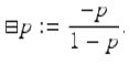
(3.10)
The fact that the addition is associative and commutative is Exercise 3.4. □
We can now define box minus subtraction,  on in a standard manner as follows.
Definition 3.9.
We define box minus subtraction on by
![$$\displaystyle{p \boxminus q:= p \boxplus [\boxminus q].}$$](fractional.files/image1606.png)
By Exercise 3.5 we have that if  , then

In addition, we define the set of (nabla) positively regressive functions,  by
by

The proof of the following theorem is left as an exercise (see Exercise 3.8).
Theorem 3.10.
The set of positively regressive functions,  , with the addition , is a subgroup of
  .
.
In the next theorem we give several properties of the exponential function E p (t, s).
Theorem 3.11.
Assume  and
and  . Then
(i)
E 0 (t,s) = 1, 
(ii)
E p (t,s) ≠ 0,
(iii)
if  , then E p (t,s) > 0,
(iv)
∇E p (t,s) = p(t)E p (t,s),  and E p (t,t) = 1,
(v)
![$$E_{p}(\rho (t),s) = [1 - p(t)]E_{p}(t,s)$$](fractional.files/image1618.png) ,
, 
(vi)
E p (t,s)E p (s,r) = E p (t,r),
(vii)

(viii)
(ix)
 .
.
Proof.
Using Example 3.7, we have that

and thus (i) holds.
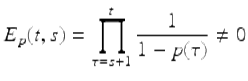
To see that (ii) holds, note that since  , it follows that 1 − p(t) ≠ 0, and hence we have that for
and for 
![$$\displaystyle{E_{p}(t,s) =\prod _{ \tau =t+1}^{s}[1 - p(\tau )]\neq 0.}$$](fractional.files/image1628.png)
Hence, (ii) holds. The proof of (iii) is similar to the proof of (ii), whereas property (iv) follows from the definition of E p (t, s).
Since, for 
![$$\displaystyle\begin{array}{rcl} E_{p}(\rho (t),s)& =& \prod _{\tau =s+1}^{t-1} \frac{1} {1 - p(\tau )} {}\\ & =& [1 - p(t)]\prod _{\tau =s+1}^{t} \frac{1} {1 - p(\tau )} {}\\ & =& [1 - p(t)]E_{p}(t,s) {}\\ \end{array}$$](fractional.files/image1630.png)
we have that (v) holds for  . Next assume
  . Then
![$$\displaystyle\begin{array}{rcl} E_{p}(\rho (t),s)& =& \prod _{\tau =\rho (t)+1}^{s}\left [1 - p(\tau )\right ] {}\\ & =& \prod _{\tau =t}^{s}\left [1 - p(\tau )\right ] {}\\ & =& [1 - p(t)]\prod _{\tau =t+1}^{s}\left [1 - p(\tau )\right ] {}\\ & =& [1 - p(t)]E_{p}(t,s). {}\\ \end{array}$$](fractional.files/image1633.png)
Hence, (v) holds for  . It is easy to check that
 ![$$E_{p}(\rho (s),s) = \left [1 - p(s)\right ]E_{p}(s,s)$$](fractional.files/image1635.png) . This completes the proof of (v).
. This completes the proof of (v).
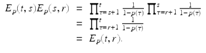
We will just show that (vi) holds when s ≥ r ≥ a. First consider the case . In this case
Next, consider the case  . Then
![$$\displaystyle\begin{array}{rcl} E_{p}(t,s)E_{p}(s,r)& =& \prod _{\tau =t+1}^{s}\left [1 - p(\tau )\right ]\prod _{\tau =r+1}^{s} \frac{1} {1 - p(\tau )} {}\\ & =& \prod _{\tau =r+1}^{t} \frac{1} {1 - p(\tau )} {}\\ & =& E_{p}(t,r). {}\\ \end{array}$$](fractional.files/image1638.png)
Finally, consider the case  . Then
![$$\displaystyle\begin{array}{rcl} E_{p}(t,s)E_{p}(s,r)& =& \prod _{\tau =t+1}^{s}\left [1 - p(\tau )\right ]\prod _{\tau =r+1}^{s} \frac{1} {1 - p(\tau )} {}\\ & =& \prod _{\tau =r+1}^{t}\left [1 - p(\tau )\right ] {}\\ & =& E_{p}(t,r). {}\\ \end{array}$$](fractional.files/image1640.png)
This completes the proof of (vi) for the special case s ≥ r ≥ a. The case a ≤ s ≤ r is left to the reader (Exercise 3.9). The proof of the law of exponents (vii) is Exercise 3.10. To see that (viii) holds, note that for 
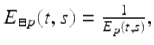
![$$\displaystyle\begin{array}{rcl} E_{\boxminus p}(t,s)& =& \prod _{\tau =s+1}^{t} \frac{1} {1 - (\boxminus p)(\tau )} {}\\ & =& \prod _{\tau =s+1}^{t}\left [1 - p(\tau )\right ] {}\\ & =& \frac{1} {E_{p}(t,s)}. {}\\ \end{array}$$](fractional.files/image1642.png)
Also, if
![$$\displaystyle\begin{array}{rcl} E_{\boxminus p}(t,s)& =& \prod _{\tau =t+1}^{s}\left [1 - (\boxminus p)(\tau )\right ] {}\\ & =& \prod _{\tau =t+1}^{s} \frac{1} {1 - p(\tau )} {}\\ & =& \frac{1} {E_{p}(t,s)}. {}\\ \end{array}$$](fractional.files/image1643.png)
Hence (viii) holds for . Finally, using (viii) and then (vii), we have that
![$$\displaystyle{ \frac{E_{p}(t,s)} {E_{q}(t,s)} = E_{p}(t,s)E_{\boxminus q}(t,s) = E_{p\boxplus [\boxminus q]}(t,s) = E_{p\boxminus q}(t,s), }$$](fractional.files/image1644.png)
from which it follows that (ix) holds. □
Next we define the scalar box dot multiplication,  .
.
Definition 3.12.
For  the scalar box dot multiplication,
  , is defined by

It follows that for 
![$$\displaystyle\begin{array}{rcl} 1 - (\alpha \boxdot p)(t)& =& 1 -\left \{1 -\left [1 - p(t)\right ]^{\alpha }\right \} {}\\ & =& \left [1 - p(t)\right ]^{\alpha } > 0 {}\\ \end{array}$$](fractional.files/image1650.png)
for . Hence  .
.
Now we can prove the following law of exponents.
Theorem 3.13.
If  and , then

for .
Proof.
Consider that, for ,
![$$\displaystyle\begin{array}{rcl} E_{p}^{\alpha }(t,a)& =& \left [\prod _{\tau =a+1}^{t} \frac{1} {1 + p(\tau )}\right ]^{\alpha } {}\\ & =& \prod _{\tau =a+1}^{t} \frac{1} {[1 + p(\tau )]^{\alpha }} {}\\ & =& \prod _{\tau =a+1}^{t} \frac{1} {1 - [1 - (1 - p(\tau ))^{\alpha }]} {}\\ & =& \prod _{\tau =a+1}^{t} \frac{1} {1 - [\alpha \boxdot p](\tau )} {}\\ & =& E_{\alpha \boxdot p}(t,a). {}\\ \end{array}$$](fractional.files/image1654.png)
This completes the proof. □
Theorem 3.14.
The set of positively regressive functions , with the addition  and the scalar multiplication
  , is a vector space.
Proof.
From Theorem 3.10 we know that with the addition is an Abelian group. The four remaining nontrivial properties of a vector space are the following:
(i)

(ii)

(iii)

(iv)

where  and
and  . We will prove properties (i)–(iii) and leave property (iv) as an exercise (Exercise 3.12).
Property (i) follows immediately from the following:

To prove (ii) consider
![$$\displaystyle\begin{array}{rcl} & & (\alpha \boxdot p) \boxplus (\alpha \boxdot q) {}\\ & & \qquad \qquad =\alpha \boxdot p +\alpha \boxdot q - (\alpha \boxdot p)(\alpha \boxdot q) {}\\ & & \qquad \qquad = [1 - (1 - p)^{\alpha }] + [1 - (1 - q)^{\alpha }] - [1 - (1 - p)^{\alpha }][1 - (1 - q)^{\alpha }] {}\\ & & \qquad \qquad = 1 - (1 - p)^{\alpha }(1 - q)^{\alpha } {}\\ & & \qquad \qquad = 1 - (1 - p - q + pq)^{\alpha } {}\\ & & \qquad \qquad = 1 - (1 - p \boxplus q)^{\alpha } {}\\ & & \qquad \qquad =\alpha \boxdot (p \boxplus q). {}\\ \end{array}$$](fractional.files/image1664.png)
Hence, (ii) holds. Finally, consider
![$$\displaystyle\begin{array}{rcl} \alpha \boxdot (\beta \boxplus p)& =& 1 - (1 -\beta \boxdot p)^{\alpha } {}\\ & =& 1 -\bigg [1 -\left [1 - (1 - p)^{\beta }\right ]\bigg]^{\alpha } {}\\ & =& 1 - (1 - p)^{\alpha \beta } {}\\ & =& (\alpha \beta ) \boxdot p. {}\\ \end{array}$$](fractional.files/image1665.png)
Hence, property (iii) holds. □