Discrete Fractional Calculus (2015)
3. Nabla Fractional Calculus
3.5. Second Order Linear Equations with Constant Coefficients
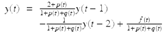
The nonhomogeneous second order linear nabla difference equation is given by
![]()
(3.12)
where we assume ![]() and
and ![]() for
for ![]() . In this section we will see that we can easily solve the corresponding second order linear homogeneous nabla difference equation with constant coefficients
. In this section we will see that we can easily solve the corresponding second order linear homogeneous nabla difference equation with constant coefficients
![]()
(3.13)
where we assume the constants ![]() satisfy
satisfy ![]() .
.
First we prove an existence-uniqueness theorem for solutions of initial value problems (IVPs) for (3.12).
Theorem 3.20.
Assume that ![]() ,
, ![]() ,
, ![]() ,
, ![]() and
and ![]() . Then the IVP
. Then the IVP
![]()
(3.14)
![]()
(3.15)
where ![]() and
and ![]() has a unique solution y(t) on
has a unique solution y(t) on ![]() .
.
Proof.
Expanding equation (3.14) we have by first solving for y(t) and then solving for y(t − 2) that, since ![]() ,
,
(3.16)
and
![]()
(3.17)
If we let ![]() in (3.16), then equation (3.14) holds at
in (3.16), then equation (3.14) holds at ![]() iff
iff
![$$\displaystyle\begin{array}{rcl} y(t_{0} + 1)& =& \frac{[2 + p(t_{0} + 1)]B} {1 + p(t_{0} + 1) + q(t_{0} + 1)} - \frac{A} {1 + p(t_{0} + 1) + q(t_{0} + 1)} {}\\ & & + \frac{f(t_{0} + 1)} {1 + p(t_{0} + 1) + q(t_{0} + 1)}. {}\\ \end{array}$$](fractional.files/image1705.png)
Hence, the solution of the IVP (3.14), (3.15) is uniquely determined at t 0 + 1. But using the equation (3.16) evaluated at ![]() , we have that the unique values of the solution at t 0 and t 0 + 1 uniquely determine the value of the solution at t 0 + 2. By induction we get that the solution of the IVP (3.14), (3.15) is uniquely determined on
, we have that the unique values of the solution at t 0 and t 0 + 1 uniquely determine the value of the solution at t 0 + 2. By induction we get that the solution of the IVP (3.14), (3.15) is uniquely determined on ![]() . On the other hand if t 0 ≥ a + 2, then using equation (3.17) with t = t 0, we have that
. On the other hand if t 0 ≥ a + 2, then using equation (3.17) with t = t 0, we have that
![]()
Hence the solution of the IVP (3.14), (3.15) is uniquely determined at t 0 − 2. Similarly, if t 0 − 3 ≥ a, then the value of the solution at t 0 − 2 and at t 0 − 1 uniquely determines the value of the solution at t 0 − 3. Proceeding in this manner we have by mathematical induction that the solution of the IVP (3.14), (3.15) is uniquely determined on ![]() . Hence the result follows. □
. Hence the result follows. □
Remark 3.21.
Note that the so-called initial conditions in (3.15)
![]()
hold iff the equations y(t 0) = C, ![]() are satisfied. Because of this we also say that
are satisfied. Because of this we also say that
![]()
are initial conditions for solutions of equation (3.12). In particular, Theorem 3.20 holds if we replace the conditions (3.15) by the conditions
![]()
Remark 3.22.
From Exercise 3.21 we see that if ![]() ,
, ![]() , then the general solution of the linear homogeneous equation
, then the general solution of the linear homogeneous equation
![]()
is given by
![]()
where y 1(t), y 2(t) are any two linearly independent solutions of (3.13) on ![]() .
.
Next we show we can solve the second order linear nabla difference equation with constant coefficients (3.13). We say the equation
![]()
is the characteristic equation of the nabla linear difference equation (3.13) and the solutions of this characteristic equation are called the characteristic values of (3.13).
Theorem 3.23 (Distinct Roots).
Assume ![]() and
and ![]() (possibly complex) are the characteristic values of (3.13) . Then
(possibly complex) are the characteristic values of (3.13) . Then
![]()
is a general solution of (3.13) on ![]() .
.
Proof.
Since ![]() ,
, ![]() satisfy the characteristic equation for (3.13), we have that the characteristic polynomial for (3.13) is given by
satisfy the characteristic equation for (3.13), we have that the characteristic polynomial for (3.13) is given by
![]()
and hence
![]()
Since
![]()
we have that ![]() and hence
and hence ![]() and
and ![]() are well defined. Next note that
are well defined. Next note that
![$$\displaystyle\begin{array}{rcl} & & \nabla ^{2}E_{\lambda _{ i}}(t,a) + p\;\nabla E_{\lambda _{i}}(t,a) + q\;E_{\lambda _{i}}(t,a) {}\\ & & \qquad \qquad \quad = [\lambda _{i}^{2} + p\lambda _{ i} + q]E_{\lambda _{i}}(t,a) {}\\ & & \qquad \qquad \quad = 0, {}\\ \end{array}$$](fractional.files/image1727.png)
for i = 1, 2. Hence ![]() , i = 1, 2 are solutions of (3.13). Since
, i = 1, 2 are solutions of (3.13). Since ![]() , these two solutions are linearly independent on
, these two solutions are linearly independent on ![]() , and by Remark 3.22,
, and by Remark 3.22,
![]()
is a general solution of (3.13) on ![]() . □
. □
Example 3.24.
Solve the nabla linear difference equation
![]()
The characteristic equation is
![]()
and the characteristic roots are
![]()
Note that ![]() , so we can apply Theorem 3.23. Then we have that
, so we can apply Theorem 3.23. Then we have that
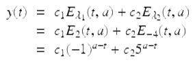
is a general solution on ![]() .
.
Usually, we want to find all real-valued solutions of (3.13). When a characteristic value ![]() of (3.13) is complex,
of (3.13) is complex, ![]() is a complex-valued solution. In the next theorem we show how to use this complex-valued solution to find two linearly independent real-valued solutions on
is a complex-valued solution. In the next theorem we show how to use this complex-valued solution to find two linearly independent real-valued solutions on ![]() .
.
Theorem 3.25 (Complex Roots).
Assume the characteristic values of (3.13) are ![]() , β > 0 and α ≠ 1. Then a general solution of (3.13) is given by
, β > 0 and α ≠ 1. Then a general solution of (3.13) is given by
![]()
where ![]() .
.
Proof.
Since the characteristic roots are ![]() , β > 0, we have that the characteristic equation is given by
, β > 0, we have that the characteristic equation is given by
![]()
It follows that ![]() and
and ![]() , and hence
, and hence
![]()
Hence, Remark 3.22 applies. By the proof of Theorem 3.23, we have that ![]() is a complex-valued solution of (3.13). Using
is a complex-valued solution of (3.13). Using
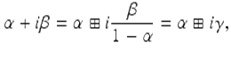
where ![]() , α ≠ 1, we get that
, α ≠ 1, we get that
![]()
is a nontrivial solution. It follows from Euler’s formula (3.11) that
![$$\displaystyle\begin{array}{rcl} y(t)& =& E_{\alpha }(t,a)E_{i\gamma }(t,a) {}\\ & =& E_{\alpha }(t,a)[\mbox{ Cos}_{\gamma }(t,a) + i\mbox{ Sin}_{\gamma }(t,a)] {}\\ & =& y_{1}(t) + iy_{2}(t) {}\\ \end{array}$$](fractional.files/image1747.png)
is a solution of (3.13). But since p and q are real, we have that the real part, y 1(t) = E α (t, a)Cos γ (t, a), and the imaginary part, y 2(t) = E α (t, a)Sin γ (t, a), of y(t) are solutions of (3.13). But y 1(t), y 2(t) are linearly independent on ![]() , so we get that
, so we get that
![]()
is a general solution of (3.13) on ![]() . □
. □
Example 3.26.
Solve the nabla difference equation
![]()
(3.18)
The characteristic equation is
![]()
and so, the characteristic roots are ![]() . Note that
. Note that ![]() . So, applying Theorem 3.25, we find that
. So, applying Theorem 3.25, we find that
![]()
is a general solution of (3.18) on ![]() .
.
The previous theorem (Theorem 3.25) excluded the case when the characteristic roots of (3.13) are 1 ± i β, where β > 0. The next theorem considers this case.
Theorem 3.27.
If the characteristic values of (3.13) are 1 ± iβ, where β > 0, then a general solution of (3.13) is given by
![]()
![]() .
.
Proof.
Since 1 − i β is a characteristic value of (3.13), we have that ![]() is a complex-valued solution of (3.13). Now
is a complex-valued solution of (3.13). Now
![$$\displaystyle\begin{array}{rcl} y(t)& =& E_{1-i\beta }(t,a) {}\\ & =& (i\beta )^{a-t} {}\\ & =& \left (\beta e^{i \frac{\pi }{2} }\right )^{a-t} {}\\ & =& \beta ^{a-t}e^{i \frac{\pi }{2} (a-t)} {}\\ & =& \beta ^{a-t}\left \{\cos \left [ \frac{\pi } {2}(a - t)\right ] + i\sin \left [ \frac{\pi } {2}(a - t)\right ]\right \} {}\\ & =& \beta ^{a-t}\cos \left [ \frac{\pi } {2}(t - a)\right ] - i\beta ^{a-t}\sin \left [ \frac{\pi } {2}(t - a)\right ]. {}\\ & & {}\\ \end{array}$$](fractional.files/image1756.png)
It follows that
![]()
are solutions of (3.13). Since these solutions are linearly independent on ![]() , we have that
, we have that
![]()
is a general solution of (3.13). □
Example 3.28.
Solve the nabla linear difference equation
![]()
The characteristic equation is ![]() , so the characteristic roots are
, so the characteristic roots are ![]() . It follows from Theorem 3.27 that
. It follows from Theorem 3.27 that
![]()
for ![]() .
.
Theorem 3.29 (Double Root).
Assume ![]() is a double root of the characteristic equation. Then
is a double root of the characteristic equation. Then
![]()
is a general solution of (3.13) .
Proof.
Since ![]() is a double root of the characteristic equation, we have that
is a double root of the characteristic equation, we have that ![]() is the characteristic equation. It follows that
is the characteristic equation. It follows that ![]() and q = r 2. Therefore
and q = r 2. Therefore
![]()
since r ≠ 1. Hence, Remark 3.22 applies. Since r ≠ 1 is a characteristic root, we have that y 1(t) = E r (t, a) is a nontrivial solution of (3.13). From Exercise 3.14, we have that ![]() is a second solution of (3.13) on
is a second solution of (3.13) on ![]() . Since these two solutions are linearly independent on
. Since these two solutions are linearly independent on ![]() , we have from Remark 3.22 that
, we have from Remark 3.22 that
![]()
is a general solution of (3.13). □
Example 3.30.
Solve the nabla difference equation
![]()
The corresponding characteristic equation is
![]()
Hence ![]() is a double root, so by Theorem 3.29 a general solution is given by
is a double root, so by Theorem 3.29 a general solution is given by
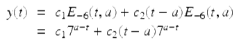
for ![]() .
.