Discrete Fractional Calculus (2015)
1. Basic Difference Calculus
1.2. Delta Exponential Function
In this section we want to study the delta exponential function that plays a similar role in the delta calculus on ![]() that the exponential function e pt ,
that the exponential function e pt , ![]() , does in the continuous calculus. Keep in mind that when p is a constant, x(t) = e pt is the unique solution of the initial value problem
, does in the continuous calculus. Keep in mind that when p is a constant, x(t) = e pt is the unique solution of the initial value problem
![]()
For the delta exponential function we would like to consider functions in the set of regressive functions defined by
![]()
Some of the results that we give will be true if in the definition of regressive functions we consider complex-valued functions instead of real-valued functions. We leave it to the reader to note when this is true.
We then define the delta exponential function corresponding to a function ![]() , based at
, based at ![]() , to be the unique solution (why does
, to be the unique solution (why does ![]() guarantee uniqueness?), e p (t, s), of the initial value problem
guarantee uniqueness?), e p (t, s), of the initial value problem
![]()
(1.4)
![]()
(1.5)
Theorem 1.11.
Assume ![]() and
and ![]() Then
Then
![$$\displaystyle{ e_{p}(t,s) = \left \{\begin{array}{@{}l@{\quad }l@{}} \prod _{\tau =s}^{t-1}[1 + p(\tau )],\quad t \in \mathbb{N}_{s} \quad \\ \prod _{\tau =t}^{s-1}[1 + p(\tau )]^{-1},\quad t \in \mathbb{N}_{a}^{s-1}.\quad \end{array} \right. }$$](fractional.files/image073.png)
(1.6)
Here, by a standard convention on products, it is understood that for any function h that
Proof.
We solve the IVP (1.4), (1.5) to get a formula for e p (t, s). Solving (1.4) for x(t + 1) we get
![]()
(1.7)
Letting t = s in (1.7) and using the initial condition (1.5) we get
![]()
Next, letting t = s + 1 in (1.7) we get
![]()
Proceeding in this fashion we get
![$$\displaystyle{ e_{p}(t,s) =\prod _{ \tau =s}^{t-1}[1 + p(\tau )] }$$](fractional.files/image078.png)
(1.8)
for ![]() . In the product in (1.8), it is understood that the index τ takes on the values
. In the product in (1.8), it is understood that the index τ takes on the values ![]() By convention
By convention ![]() . Next assume
. Next assume ![]() . Solving (1.7) for x(t) we get
. Solving (1.7) for x(t) we get
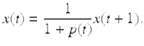
(1.9)
Letting t = s − 1 in (1.9), we get
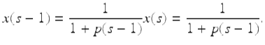
Next, letting t = s − 2 in (1.9), we get
![$$\displaystyle{x(s - 2) = \frac{1} {1 + p(s - 2)}x(s - 1) = \frac{1} {\left [1 + p(s - 2)\right ]\left [1 + p(s - 1)\right ]}.}$$](fractional.files/image085.png)
Continuing in this manner we get
![$$\displaystyle{x(t) =\prod _{ \tau =t}^{s-1}[1 + p(\tau )]^{-1},\quad t \in \mathbb{N}_{ a}^{s-1}.}$$](fractional.files/image086.png)
□
Theorem 1.11 gives us the following example.
Example 1.12.
If p(t) = p is a constant with p ≠ − 1 (note this constant function is in ![]() ), then from (1.6)
), then from (1.6)
![]()
Example 1.13.
Find e p (t, 1) if p(t) = t − 1, ![]() First note that 1 + p(t) = t ≠ 0 for
First note that 1 + p(t) = t ≠ 0 for ![]() , so
, so ![]() . From (1.6) we get
. From (1.6) we get
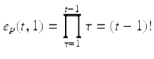
for ![]() .
.
It is easy to prove the following theorem.
Theorem 1.14.
If ![]() , then a general solution of
, then a general solution of
![]()
is given by
![]()
where c is an arbitrary constant.
The following example is an interesting application using an exponential function.
Example 1.15.
According to folklore, Peter Minuit in 1626 purchased Manhattan Island for goods worth $24. If at the beginning of 1626 the $24 could have been invested at an annual interest rate of 7% compounded quarterly, what would it have been worth at the end of the year 2014. Let y(t) be the value of the investment after t quarters of a year. Then y(t) satisfies the equation
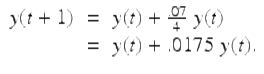
Thus y is a solution of the IVP
![]()
Using Theorem 1.14 and the initial condition we get that
![]()
It follows that
![]()
(about 11.8 trillion dollars!).
We now develop some properties of the (delta) exponential function e p (t, a). To motivate our later results, consider, for ![]() the product
the product
![$$\displaystyle\begin{array}{rcl} e_{p}(t,a)e_{q}(t,a)& =& \prod _{\tau =a}^{t}(1 + p(\tau ))\prod _{\tau =a}^{t}(1 + q(\tau )) {}\\ & =& \prod _{\tau =a}^{t}[1 + p(\tau )][1 + q(\tau )] {}\\ & =& \prod _{\tau =a}^{t}[1 + (p(t) + q(t) + p(t)q(t))] {}\\ & =& \prod _{\tau =a}^{t}[1 + (p \oplus q)(\tau )],\quad \mbox{ if $(p \oplus q)(t):= p(t) + q(t) + p(t)q(t)$} {}\\ & =& e_{p\oplus q}(t,a). {}\\ \end{array}$$](fractional.files/image100.png)
Hence we get the law of exponents
![]()
holds for ![]() provided
provided
![]()
Theorem 1.16.
If we define the circle plus addition , ⊕, on ![]() by
by
![]()
then ![]() , ⊕ is an Abelian group.
, ⊕ is an Abelian group.
Proof.
First to see the closure property is satisfied, note that if ![]() , then 1 + p(t) ≠ 0 and 1 + q(t) ≠ 0 for
, then 1 + p(t) ≠ 0 and 1 + q(t) ≠ 0 for ![]() It follows that
It follows that
![]()
for ![]() and hence
and hence ![]() .
.
Next the zero function ![]() as 1 + 0 = 1 ≠ 0. Also
as 1 + 0 = 1 ≠ 0. Also
![]()
so the zero function 0 is the additive identity element in ![]()
To show that every element in ![]() has an additive inverse let
has an additive inverse let ![]() . Then set
. Then set ![]() and note that since
and note that since
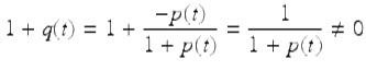
for ![]() , so
, so ![]() and we also have that
and we also have that
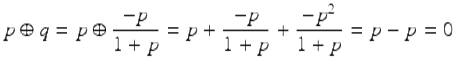
so q is the additive inverse of p. For ![]() we use the following notation for the additive inverse of p:
we use the following notation for the additive inverse of p:
![]()
(1.10)
The fact that the addition ⊕ is associative and commutative is Exercise 1.19. □
We can now define circle minus subtraction on ![]() in the standard way that subtraction is defined in terms of addition.
in the standard way that subtraction is defined in terms of addition.
Definition 1.17.
We define circle minus subtraction on ![]() by
by
![]()
It can be shown (Exercise 1.18) that if ![]() then
then

The next theorem gives us several properties of the exponential function e p (t, s), based at ![]() .
.
Theorem 1.18.
Assume ![]() and
and ![]() . Then
. Then
(i)
e 0 (t,s) = 1 and e p (t,t) = 1;
(ii)
![]()
(iii)
if 1 + p > 0, then e p (t,s) > 0;
(iv)
![]()
(v)
![]()
(vi)
e p (t,s)e p (s,r) = e p (t,r);
(viii)
e p (t,s)e q (t,s) = e p⊕q (t,s);
(viii)
![]()
(ix)
![]()
(x)
![]()
Proof.
We prove many of these properties when s = a and leave it to the reader to show that the same results hold for any ![]() . By the definition of the exponential we have that (i) and (iv) hold. To see that (ii) holds when s = a note that since
. By the definition of the exponential we have that (i) and (iv) hold. To see that (ii) holds when s = a note that since ![]() , 1 + p(t) ≠ 0 for
, 1 + p(t) ≠ 0 for ![]() and hence we have that
and hence we have that
![$$\displaystyle{e_{p}(t,a) =\prod _{ \tau =a}^{t-1}[1 + p(\tau )]\neq 0,}$$](fractional.files/image136.png)
for ![]() . The proof of (iii) is similar to the proof of (ii).
. The proof of (iii) is similar to the proof of (ii).
Since
![$$\displaystyle\begin{array}{rcl} e_{p}(\sigma (t),a)& =& \prod _{\tau =a}^{\sigma (t)-1}[1 + p(\tau )] {}\\ & =& \prod _{\tau =a}^{t}[1 + p(\tau )] {}\\ & =& [1 + p(t)]e_{p}(t,a), {}\\ \end{array}$$](fractional.files/image137.png)
we have that (v) holds when s = a.
We only show (vi) holds when t ≥ s ≥ r and leave the other cases to the reader. In particular, we merely observe that
![$$\displaystyle\begin{array}{rcl} e_{p}(t,s)e_{p}(s,r)& =& \prod _{\tau =s}^{t-1}[1 + p(\tau )]\prod _{\tau =r}^{s-1}[1 + p(\tau )] {}\\ & =& \prod _{\tau =r}^{t-1}[1 + p(\tau )] {}\\ & =& e_{p}(t,r). {}\\ \end{array}$$](fractional.files/image138.png)
We proved (vii) holds when with s = a, earlier to motivate the definition of the circle plus addition. To see that (viii) holds with s = a note that
![$$\displaystyle\begin{array}{rcl} e_{\ominus p}(t,a)& =& \prod _{\tau =a}^{t-1}[1 + (\ominus p)(\tau )] {}\\ & =& \prod _{\tau =a}^{t-1} \frac{1} {1 + p(\tau )} {}\\ & =& \frac{1} {\prod _{\tau =a}^{t-1}[1 + p(\tau )]} {}\\ & =& \frac{1} {e_{p}(t,a)}. {}\\ \end{array}$$](fractional.files/image139.png)
Since
![$$\displaystyle{ \frac{e_{p}(t,a)} {e_{q}(t,a)} = e_{p}(t,a)e_{\ominus q}(t,a) = e_{p\oplus [\ominus q]}(t,a) = e_{p\ominus q}(t,a), }$$](fractional.files/image140.png)
we have (ix) holds when s = a. Since
![$$\displaystyle{e_{p}(t,a) =\prod _{ s=a}^{t-1}[1 + p(s)] = \frac{1} {\prod _{s=a}^{t-1}[1 + p(s)]^{-1}} = \frac{1} {e_{p}(a,t)},}$$](fractional.files/image141.png)
we have that (x) holds. □
Before we derive some other properties of the exponential function we give another example where we use an exponential function.
Example 1.19.
Assume initially that the number of bacteria in a culture is P 0 and after one hour the number of bacteria present is ![]() . Find the number of bacteria, P(t), present after t hours. How long does it take for the number of bacteria to triple? Experiments show that P(t) satisfies the IVP (why is this plausible?)
. Find the number of bacteria, P(t), present after t hours. How long does it take for the number of bacteria to triple? Experiments show that P(t) satisfies the IVP (why is this plausible?)
![]()
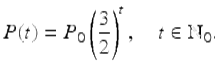
Solving this IVP we get from Theorem 1.14 that
![]()
Using the fact that ![]() we get
we get ![]() . It follows that
. It follows that
Let t 0 be the amount of time it takes for the population of the bacteria to triple. Then
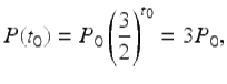
which implies that
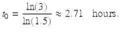
The set of positively regressive functions, ![]() , is defined by
, is defined by
![]()
Note that by Theorem 1.18, part (iii), we have that if ![]() , then e p (t, a) > 0 for
, then e p (t, a) > 0 for ![]() . It is easy to see (Exercise 1.20) that
. It is easy to see (Exercise 1.20) that ![]() is a subgroup of
is a subgroup of ![]() .
.
We next define the circle dot scalar multiplication ⊙ on ![]()
Definition 1.20.
The circle dot scalar multiplication, ⊙, is defined on ![]() by
by
![]()
Theorem 1.21.
If ![]() and
and ![]() , then
, then
![]()
for ![]()
Proof.
Consider
![$$\displaystyle\begin{array}{rcl} e_{p}^{\alpha }(t,a)& =& \left \{\prod _{\tau =a}^{t-1}[1 + p(\tau )]\right \}^{\alpha } {}\\ & =& \prod _{\tau =a}^{t-1}[1 + p(\tau )]^{\alpha } {}\\ & =& \prod _{\tau =a}^{t-1}\{1 + [(1 + p(\tau ))^{\alpha } - 1]\} {}\\ & =& \prod _{\tau =a}^{t-1}[1 + (\alpha \odot p)(\tau )] {}\\ & =& e_{\alpha \odot p}(t,a). {}\\ \end{array}$$](fractional.files/image160.png)
This completes the proof. □
The following lemma will be used in the proof of the next theorem.
Lemma 1.22.
If ![]() and
and
![]()
then p = q.
Proof.
Assume ![]() and e p (t, a) = e q (t, a) for
and e p (t, a) = e q (t, a) for ![]() It follows that
It follows that
![]()
Dividing by e p (t, a) = e q (t, a) we get that p = q. □
Theorem 1.23.
The set of positively regressive functions ![]() , with the addition ⊕, and the scalar multiplication ⊙ is a vector space.
, with the addition ⊕, and the scalar multiplication ⊙ is a vector space.
Proof.
We just prove two of the properties of a vector space and leave the rest of the proof (see Exercise 1.25) to the reader. First we show that the distributive law
![]()
holds for ![]() ,
, ![]() This follows from
This follows from
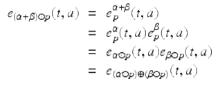
and an application of Lemma 1.22. Next we show that 1 ⊙ p = p for all ![]() This follows from
This follows from
![]()
and an application of Lemma 1.22. □