Discrete Fractional Calculus (2015)
3. Nabla Fractional Calculus
3.8. Nabla Taylor’s Theorem
In this section we want to prove the nabla version of Taylor’s Theorem. To do this we first study the nabla Taylor monomials and give some of their important properties. These nabla Taylor monomials will appear in the nabla Taylor’s Theorem. We then will find nabla Taylor series expansions for the nabla exponential, hyperbolic, and trigonometric functions. Finally, as a special case of our Taylor’s theorem we will obtain a variation of constants formula for ∇ n y(t) = h(t).
Definition 3.46.
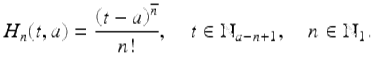
We define the nabla Taylor monomials , H n (t, a), ![]() , by H 0(t, a) = 1, for
, by H 0(t, a) = 1, for ![]() , and
, and
Theorem 3.47.
The nabla Taylor monomials satisfy the following:
(i)
![]()
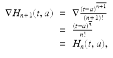
(ii)
![]()
(iii)
![]()
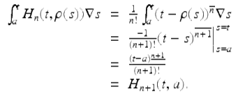
(iv)
![]() .
.
Proof.
Part (i) of this theorem follows from the definition (Definition 3.46) of the nabla Taylor monomials. By the first power rule (3.3), it follows that
and so, we have that part (ii) of this theorem holds. Part (iii) follows from parts (ii) and (i). Finally, to see that (iv) holds we use the integration formula in part (iii) in Theorem 3.36 to get
This completes the proof. □
Now we state and prove the nabla Taylor’s Theorem.
Theorem 3.48 (Nabla Taylor’s Formula).
Assume ![]() where
where ![]() . Then
. Then
![]()
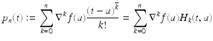
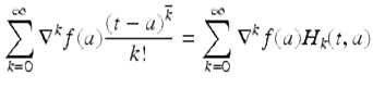
where the n-th degree nabla Taylor polynomial, p n (t), is given by
and the Taylor remainder, R n (t), is given by
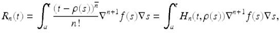
for ![]() . (By convention we assume R n (t) = 0 for a − n ≤ t < a.)
. (By convention we assume R n (t) = 0 for a − n ≤ t < a.)
Proof.
We will use the second integration by parts formula in Theorem 3.39, namely (3.20), to evaluate the integral in the definition of R n (t). To do this we set
![]()
Then it follows that
![]()
Using part (iv) of Theorem 3.47, we get
![]()
Hence we get from the second integration by parts formula (3.20) that
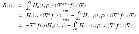
Again, using the second integration by parts formula (3.20), we have that
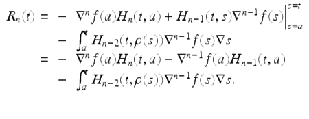
By induction on n we obtain
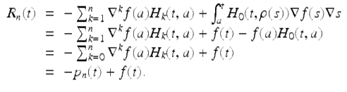
Solving for f(t) we get the desired result. □
We next define the formal nabla power series of a function at a point.
Definition 3.49.
Let ![]() and let
and let
![]()
If ![]() , then we call
, then we call
the (formal) nabla Taylor series of f at t = a
The following theorem gives some convergence results for nabla Taylor series for various functions.
Theorem 3.50.
Assume |p| < 1 is a constant. Then the following hold:
(i)
![]()
(ii)
![]()
(iii)
![]()
(iv)
![]()
(v)
![]()
for ![]() .
.
Proof.
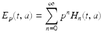
First we prove part (i). Since ![]() for
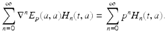
for ![]() , we have that the Taylor series for E p (t, a) is given by
, we have that the Taylor series for E p (t, a) is given by
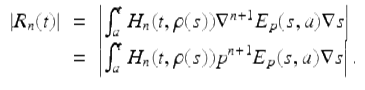
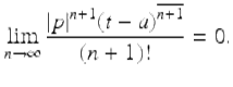
To show that the above Taylor series converges to E p (t, a) when | p | < 1 is a constant, for each ![]() , it suffices to show that the remainder term, R n (t), in Taylor’s Formula satisfies
, it suffices to show that the remainder term, R n (t), in Taylor’s Formula satisfies
![]()
when | p | < 1, for each fixed ![]() ,
,
So fix ![]() and consider
and consider
Since t is fixed, there is a constant C such that
![]()
Hence,

By the ratio test, if | p | < 1, the series
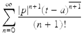
converges. It follows that if | p | < 1, then by the n-th term test
This implies that if | p | < 1, then for each fixed ![]()
![]()
and hence if | p | < 1,
for all ![]() . Since the functions Sin p (t, a), Cos p (t, a), Sinh p (t, a), and Cosh p (t, a) are defined in terms of E p (t, a), parts (ii)–(v) follow easily from part (i). □
. Since the functions Sin p (t, a), Cos p (t, a), Sinh p (t, a), and Cosh p (t, a) are defined in terms of E p (t, a), parts (ii)–(v) follow easily from part (i). □
We now see that the integer order variation of constants formula follows from Taylor’s formula.
Theorem 3.51 (Integer Order Variation of Constants Formula).
Assume ![]() and
and ![]() . Then the solution of the IVP
. Then the solution of the IVP
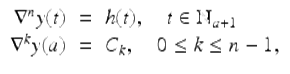
(3.29)
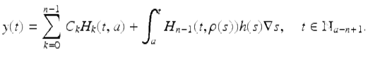
where C k , 0 ≤ k ≤ n − 1, are given constants, is given by the variation of constants formula
Proof.
It is easy to see that the given IVP has a unique solution y that is defined on ![]() . By Taylor’s formula (see Theorem 3.48) with n replaced by n − 1 we get that
. By Taylor’s formula (see Theorem 3.48) with n replaced by n − 1 we get that
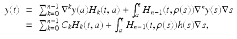
![]() . □
. □
We immediately get the following special case of Theorem 3.51. This special case, which we label Corollary 3.52, is also called a variation of constants formula.
Corollary 3.52 (Integer Order Variation of Constants Formula).
Assume the function ![]() and
and ![]() . Then the solution of the IVP
. Then the solution of the IVP
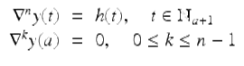
(3.30)
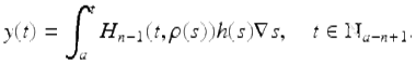
is given by the variation of constants formula.
Example 3.53.
Use the variation of constants formula to solve the IVP
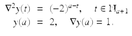
By the variation of constants formula in Theorem 3.51 the solution of this IVP is given by
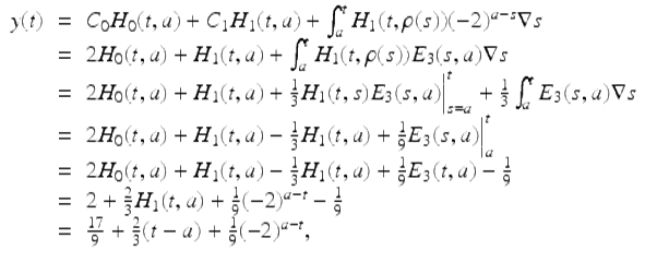
for ![]() .
.