Discrete Fractional Calculus (2015)
3. Nabla Fractional Calculus
3.10. Nabla Laplace Transforms
Having established the necessary preliminaries, we are now ready to discuss an important application of this material: the Laplace transform. The Laplace transform, as in the standard calculus, will provide us with an elegant way to solve initial value problems for a fractional nabla difference equation. In this section, we will lay the groundwork for this method, prove the basic properties, and establish a means in which to solve various initial value (nabla) fractional difference equations. We begin this section by defining the nabla Laplace transform operator ![]() (based at a) as follows:
(based at a) as follows:
Definition 3.64.
Assume ![]() . Then the nabla Laplace transform of f is defined by
. Then the nabla Laplace transform of f is defined by
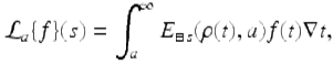
for those values of s ≠ 1 such that this improper integral converges.
In the following theorem we give another formula for the Laplace transform, which is often more convenient to use.
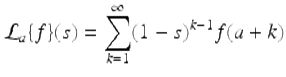
Theorem 3.65.
Assume ![]() . Then
. Then
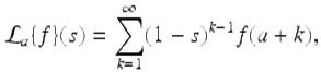
(3.36)
for those values of s such that this infinite series converges.
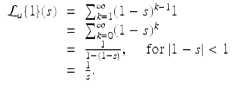
Proof.
Assume ![]() . Then
. Then
![$$\displaystyle\begin{array}{rcl} \mathcal{L}_{a}\{f\}(s)& =& \int _{a}^{\infty }E_{ \boxminus s}(\rho (t),a)f(t)\nabla t {}\\ & =& \int _{a}^{\infty }[1 -\boxminus s]^{a-t+1}f(t)\nabla t {}\\ & =& \int _{a}^{\infty }\left ( \frac{1} {1 - s}\right )^{a-t+1}f(t)\nabla t {}\\ & =& \int _{a}^{\infty }(1 - s)^{t-a-1}f(t)\nabla t {}\\ & =& \sum _{t=a+1}^{\infty }(1 - s)^{t-a-1}f(t) {}\\ & =& \sum _{k=1}^{\infty }(1 - s)^{k-1}f(a + k), {}\\ \end{array}$$](fractional.files/image1969.png)
for those values of s such that this infinite series converges. □
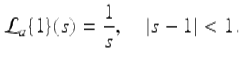
In the definition of the nabla Laplace transform we assumed s ≠ 1 because we do not define ![]() . But the formula of the nabla Laplace transform (3.36) is well defined when s = 1. From now on we will always include s = 1 in the domain of convergence for the nabla Laplace transform although in the proofs we will often assume s ≠ 1. In fact the formula (3.36) for any
. But the formula of the nabla Laplace transform (3.36) is well defined when s = 1. From now on we will always include s = 1 in the domain of convergence for the nabla Laplace transform although in the proofs we will often assume s ≠ 1. In fact the formula (3.36) for any ![]() gives us that
gives us that
![]()
Example 3.66.
We use the last theorem to find ![]() . By Theorem 3.65 we obtain
. By Theorem 3.65 we obtain
That is
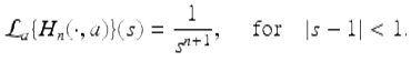
Theorem 3.67.
For all nonnegative integers n, we have that
Proof.
The proof is by induction on n. The result is true for n = 0 by the previous example. Suppose now that ![]() for some fixed n ≥ 0 and | s − 1 | < 1. Then consider
for some fixed n ≥ 0 and | s − 1 | < 1. Then consider
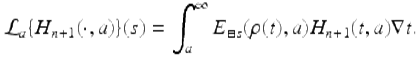
We will apply the first integration by parts formula (3.19) with
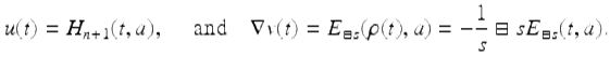
It follows that
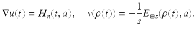
Hence by the integration by parts formula (3.19)
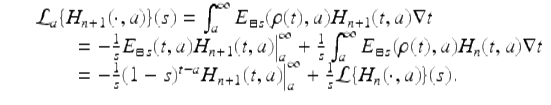
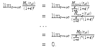
Using the nabla form of L’Hôpital’s rule (Exercise 3.19) we calculate
![$$\displaystyle\begin{array}{rcl} \lim _{t\rightarrow \infty }\vert (1 - s)^{t-a}H_{ n+1}(t,a)\vert & =& \lim _{t\rightarrow \infty }\frac{H_{n+1}(t,a)} {\vert 1 - s\vert ^{a-t}} {}\\ & =& \lim _{t\rightarrow \infty } \frac{H_{n}(t,a)} {[1 -\vert 1 - s\vert ]\vert 1 - s\vert ^{a-t}} {}\\ & =& \lim _{t\rightarrow \infty } \frac{H_{n-1}(t,a)} {[1 -\vert 1 - s\vert ]^{2}\vert 1 - s\vert ^{a-t}} {}\\ & =& \cdots {}\\ & =& \lim _{t\rightarrow \infty } \frac{H_{0}(t,a)} {[1 -\vert 1 - s\vert ]^{n+1}\vert 1 - s\vert ^{a-t}} {}\\ & =& 0, {}\\ \end{array}$$](fractional.files/image1982.png)
since | s − 1 | < 1. Thus we have that
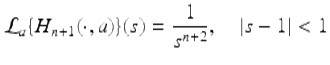
completing the proof. □
Definition 3.68.
A function ![]() is said to be of exponential order r > 0 if there exist a constant M > 0 and a number
is said to be of exponential order r > 0 if there exist a constant M > 0 and a number ![]() such that
such that
![]()
Theorem 3.69.
For ![]() , the Taylor monomials H n (t,a) are of exponential order 1 + ε for all ε > 0. Also, H 0 (t,a) is of exponential order 1.
, the Taylor monomials H n (t,a) are of exponential order 1 + ε for all ε > 0. Also, H 0 (t,a) is of exponential order 1.
Proof.
Since
![]()
H 0(t, a) is of exponential order 1. Next, assume ![]() and ε > 0 is fixed. Using repeated applications of the nabla L’Hôpital’s rule, we get
and ε > 0 is fixed. Using repeated applications of the nabla L’Hôpital’s rule, we get
It follows from this that each H n (t, a), ![]() , is of exponential order 1 +ε for all ε > 0. □
, is of exponential order 1 +ε for all ε > 0. □
Theorem 3.70 (Existence of Nabla Laplace Transform).
If ![]() is a function of exponential order r > 0, then its Laplace transform exists for
is a function of exponential order r > 0, then its Laplace transform exists for ![]() .
.
Proof.
Let f be a function of exponential order r. Then there is a constant M > 0 and a number ![]() such that | f(t) | ≤ Mr t for all
such that | f(t) | ≤ Mr t for all ![]() . Pick K so that
. Pick K so that ![]() , then we have that
, then we have that
![]()
We now show that
converges for ![]() . To see this, consider
. To see this, consider
![$$\displaystyle\begin{array}{rcl} \sum _{k=K}^{\infty }\vert (1 - s)^{k-1}f(a + k)\vert & =& \sum _{ k=K}^{\infty }\vert 1 - s\vert ^{k-1}\vert f(a + k)\vert {}\\ &\leq & \sum _{k=K}^{\infty }\vert 1 - s\vert ^{k-1}Mr^{a+k} {}\\ & =& Mr^{a+1}\sum _{ k=K}^{\infty }[r\vert s - 1\vert ]^{k-1}, {}\\ \end{array}$$](fractional.files/image1994.png)
which converges since r | s − 1 | < 1. It follows that ![]() converges absolutely for
converges absolutely for ![]() . □
. □
Theorem 3.71.
The Laplace transform of the Taylor monomial, H n (t,a), ![]() , exists for |s − 1| < 1.
, exists for |s − 1| < 1.
Proof.
The proof of this theorem follows from Theorems 3.69 and 3.70. □
Similarly, by Exercise 3.30 each of the functions E p (t, a), Cosh p (t, a), Sinh p (t, a), Cos p (t, a), and Sin p (t, a) is of exponential order | 1 + p | , and hence by Theorem 3.70 their Laplace transforms exist for ![]() .
.
Theorem 3.72 (Uniqueness Theorem).
Assume ![]() . Then f(t) = g(t),
. Then f(t) = g(t), ![]() if and only if
if and only if
![]()
for some r > 0.
Proof.
Since ![]() is a linear operator it suffices to show that f(t) = 0 for
is a linear operator it suffices to show that f(t) = 0 for ![]() if and only if
if and only if ![]() for | s − 1 | < r for some r > 0. If f(t) = 0 for
for | s − 1 | < r for some r > 0. If f(t) = 0 for ![]() , then trivially
, then trivially ![]() for all
for all ![]() . Conversely, assume that
. Conversely, assume that ![]() for | s − 1 | < r for some r > 0. In this case we have that
for | s − 1 | < r for some r > 0. In this case we have that
This implies that
![]()
This completes the proof. □