The Handy Math Answer Book, Second Edition (2012)
MATHEMATICAL ANALYSIS
ANALYSIS BASICS
What is mathematical analysis?
Mathematical analysis is a branch of mathematics that uses the concepts and methods common to the field of calculus. The key to mathematical analysis is the use of infinite processes; in turn, that involves passage to a limit, or, in other words, the basic branch of calculus. For example, a circle’s area can be thought of as the limiting value of the areas of regular polygons within the circle, as the number of the polygons’ sides increase indefinitely. The reason for calculus is simple: It is one of the most powerful and flexible tools not only in mathematics but in virtually every scientific field.
What culture took the first steps in the development of mathematical analysis?
Mathematical analysis—and, thus, the ideas of calculus—took centuries to develop. Probably the first to present some solid concepts in the field were the Greeks whose most important contribution was the method of exhaustion (expanding the measurements of an area to take in more and more of the required area).
For example, Zeno of Elea (c. 490-c. 425 B.C.E.) based many problems on the infinite; Leucippus of Miletus (fl. c. 435-c. 420 B.C.E.), Democritus of Abdera (460-370 B.C.E.; a student of Leucippus who also proposed an early theory about how the universe was formed), and Antiphon (c. 479-411 B.C.E.; who some historians believe tried to square the circle) would all contribute to the method of exhaustion. Eudoxus of Cnidus (c. 400-347 B.C.E.) would be the first to use the method on a scientific basis. Archimedes (c. 287-212 B.C.E.; Hellenic)—considered one of the greatest Greek mathematicians—took mathematical analysis one step further: He more fully developed the theory presented by Eudoxus that would eventually lead to integral calculus.
What is considered one of Archimedes’s most significant contributions to mathematics?
Archimedes made many significant contributions to mathematics, though not all mathematicians would agree with the label “most significant.” But one of his contributions did advance the field of calculus by showing that the area of a segment of a parabola is 4/3 the area of a triangle with the same base and vertex (endpoint), and 2/3 the area of the circumscribed parallelogram.
To figure this out, he constructed an “infinite” sequence of triangles (or wedges), finding the area of segments composing the parabola. He began with the first area, A, then added more triangles between the existing ones and the parabola to get areas of:
A, A + A/4, A + A/4 + A/16, A + A/4 + A/16 + A/64, and so on.
Based on his iterations, he determined the following (the first time anyone had determined the summation of an infinite series; for more about infinite series, see below):
A(1 + 1/4 + 1/42 + 1/43 + …) = A(4/3)
Archimedes also applied this method of exhaustion (not literally becoming tired, but close to it) to approximate the area of a circle, which, in turn, led to a better approximation of pi (π). Using such integrations, he also determined the volume and surface area of a sphere and cone, the surface area of an ellipse, and many others. His work is considered the first steps toward integration that would eventually lead to integral calculus. (For more information about Archimedes and his wedges, see “Geometry and Trigonometry.”)

Astronomer and mathematician Johannes Kepler used sectors to calculate the shape of the elliptical paths of the planets.
What did Isaac Newton contribute to mathematical analysis?
English mathematician and natural philosopher (otherwise called a physicist) Isaac Newton (1642–1727) was one of the greatest scientists who ever lived. Overall, he contributed to physics (such as the discovery of his three famous laws of motion); fluid dynamics (fluid motion); the union of terrestrial and celestial mechanics using the principle of gravitation—thus explaining Kepler’s laws of planetary motion; and he even explained the principle of universal gravitation.
By 1665 Newton had not only begun his work on differential calculus, but he also had published one of his greatest scientific works—Philosophiae naturalis principia mathematica (The Mathematical Principles of Natural Philosophy), often shortened to The Principia or just Principia. In it he presents his theories of motion, gravity, and mechanics, thus explaining the bizarre orbits of comets, tides and tidal variations, the movement of the Earth’s axis (called precession), and motion of the Moon. And although he used calculus to find many of his scientific results, Newton also explained them using older geometric methods in the book. After all, calculus was very new. Perhaps he was the first scientist-writer to make sure everyone understood what he was proposing.
How did mathematical analysis develop after the 16th century?
Ideas about mathematical analysis took a long hiatus after the Greeks. It didn’t begin to grow again until the 16th century, when the need to examine mechanics problems became important. For example, German astronomer and mathematician Johannes Kepler (1571–1630) needed to calculate the area of sectors in an ellipse in order to understand planetary motion. (Interestingly, Kepler thought of areas as the sums of lines—a kind of crude form of integration; even though he made two errors in his work, they canceled each other out and he was still able to determine the correct numbers.)
By the 17th century, many mathematicians had begun to contribute to the field of mathematical analysis. For example, French mathematician Pierre de Fermat (1601–1665) made contributions that eventually led to differential calculus. Bonaventura Cavalieri presented his method of indivisibles, one he developed after examining Kepler’s integration work. English mathematician Isaac Barrow (1630–1677) worked on tangents that formed the foundation for Newton’s work on calculus. Italian mathematician Evangelista Torricelli (1608–1647) added to differential calculus and many other facets of mathematical analysis. (In fact, collections of paradoxes that arose through the inappropriate use of the new calculus were found in his manuscripts. Unfortunately for mathematics, Torricelli died young of typhoid.) And, of course, the one name most associated with calculus— Isaac Newton—developed some of his most brilliant work during the 17th century.
Why was Gottfried Wilhelm Leibniz important to calculus?
German philosopher and mathematician Baron Gottfried Wilhelm Leibniz (1646–1716) was a contemporary of Isaac Newton. He is considered by some to be a forgotten mathematician, being overshadowed by Newton, but his contributions to mathematics were just as important. In addition to many other contributions, he (independently of Newton) developed infinitesimal calculus and was first to describe it in print. Because his work on calculus was published three years before Isaac Newton’s, Leibniz’s system of notation was universally adopted, including the notation for an integral. In 1684, he published Nova methodus pro maximis et minimis, itemque tangentibus, a work detailing differential calculus and containing the familiar d (or d/dx) notation, along with the rules for calculating the derivatives of powers, products, and quotients.
SEQUENCES AND SERIES
What is a sequence?
A sequence is defined as a set of real numbers with a natural order. A sequence is usually included in brackets ({}), with the terms, or parts of a sequence, separated by commas. For example, if a scientist collects weather data every day for many days, the first day of collecting can be written as x1 data; then x2 for the second day, and so on until xn, in which n is the eventual number of days. This can be written as {x1, x2, … xn} n≥1. In general, the sequence of numbers in which xn is the nth number is written using the following notation: {xn}n≥1.
A sequence can get larger or smaller. For example, in the sequence for {2n}n≥1, the solution is 2 ≤ 4 ≤ 8 ≤ 16 ≤ 32, and so on, with the numbers getting larger. Whereas, for {1/n}n≥1, the sequence becomes 1 ≥ ½ ≥ 1/3 ≥ 1/4 ≥ 1/5, and so on, with the numbers getting progressively smaller. This does not mean that sequences only get progressively larger and smaller; certain solutions for sequences include a mix of the two.
What is the range of a sequence?
The range of a sequence is merely a set that defines the sequence. The range is usually represented by the set {x1}, {x2}, {x3}, and so on; it is also written as {xn; n = 1, 2, 3, …}. For example, in the question above, the data for each day that the scientist collects from his weather experiment is the range. Another example is the range of the sequence {(-1)n}n ≥ 1: It is the two-element set {-1, 1}.
When is a sequence monotonic?
A sequence is called monotonic if one of the following properties hold: In the sequence {xn}n≥1, it is increasing if and only if xn < xn + 1 for any n ≥ 1, or it is decreasing if and only if xn > xn + 1 for any n ≥ 1.
For example, in order to check that the sequence {2n}n≥1 is increasing: Let n ≥ 1; that gives 2n+1 = 2n 2. Because 2 is greater than 1, which means that 1 × 2n < 2 × 2n; thus 2n < 2n + 1, which shows the sequence is increasing.
How can a calculator determine the limit of a sequence?
There is an excellent way to understand the limit of a sequence by using a calculator. In scientific calculators that include geometric functions (such as cosine, sine, and tangent), a limit is easy to see: Find x1 = cos (1), then x2 = cos (x1), and so on. Just put the calculator in the “radian” mode, enter “1,” and then hit the “cosine” key repeatedly. The number will start at “0.540302305,” then change to “0.857553215,” and keep changing. As it approaches about the twentieth change, the amount gets closer and closer to a number that begins as “0.73 …”. This indicates the limit of the sequence is being reached.
What are the bounds of a sequence?
Once again, take the sequence {xn}n≥1. This sequence is bounded above if and only if there is a number M such that xn ≤ M (the M is called an upper-bound). In addition, the sequence is bounded below if and only if there is a number m such that xn ≥ m (the m is called a lower-bound). For example, the sequence {2n}n≥1, is bounded below by 0 because it is positive, but not bounded above.
The sequence is usually said to be merely bounded (or “bd” for short) if both of the properties (upper- and lower-bound) hold. For example, the harmonic sequence {1, ½, 1/3, 1/4 …} is considered bounded because no term is greater than 1 or less than 0; thus, the upper- and lower-bounds, respectively, apply.
What is a limit of a sequence?
The limit of a sequence is simply the number that represents a kind of equilibrium reached in the sequence. It is also phrased “approaches as closely as possible.” (Limit is also a term used in calculus in relation to a function; see elsewhere in this chapter.)
What are the concepts of convergent and divergent sequences?
Convergent and divergent sequences are based on the limit of a sequence. A convergent sequence, the one most commonly worked on in calculus, means that one mathematical sequence gets close to another and eventually approaches a limit (convergence can also apply to curves, functions, or series). This is seen visually when a curve approaches the x or y axes but does not quite reach it. For example, take the sequence of numbers used above, or {xn}n≥1. Often the numbers come closer and closer to a number we’ll call L; written in calculus, xn ≈ L. If the numbers do come closer, the sequence is said to be convergent and has a limit equal to L. Conversely, if the sequence is not convergent, it is called divergent.
Most mathematicians and scientists are not only interested in how a sequence converges (or diverges), but also how fast it converges, which is called the speed of convergence. There are several basic properties of the limits of a sequence, including that the limit of a convergent sequence is unique, every convergent sequence is bounded, and any bounded increasing or decreasing sequence is convergent.
How are limits written in terms of convergent and divergent sequences?
Limits of convergent and divergent sequences are written as follows (the figure eight on its side is the symbol for infinity):
![]()
What is a series?
A series is closely related to the sum of numbers. It is actually used to help add numbers; therefore, in a sequence it can be the indicated sum of that sequence. In general, the idea is to start with a number, then do something to that number to get the next number, then do the same to that number to get the next number, and so on. For example, a finite series with six terms is 2 + 4 + 6 + 8 + 10 + 12, in which 2 is added to each number to get the next number. An example of an infinite series is one with the notation 1/2n, with n ≥ 1, or ½ + 1/4 + 1/8 + … (and so on).
To see a series written in notation, if set {xn} is a sequence of numbers being added, and set s1 = x1, then s2 = x1 + x2; s3 = x1 + x2 + x3; and so on. And for n ≥ 1, a new sequence is made, {sn}, called the sequence of partial sums, or sn = x1 + x2 + … + xn
What is the notation commonly used for series and sequences?
When looking at a sequence and series, we need to distinguish between the ones we want to add, and the ones we do not want to add. The common symbol used for addition with a sequence or a series is the summation symbol, seen as the symbol Σ. When discussing a series, this symbol is used to mean the sum of numbers. For example, for the series called xn:
![]()
Also note that for any given series Σxn, we have to also remember to associate it with the sequence of partial sums (sn = x1 + x2 + … + xn).
What are arithmetic series and sequences?
An arithmetic series—also called arithmetic progression—is one of the simpler types of series in mathematics. In such a series, each new term is the previous number plus a given number; it is usually seen in the form of a + (a + d) + (a + 2d) + (a + 3d) + , …, a + (n - 1)d. An example of an arithmetic series would be 2 + 6 + 10 + 14 + …, and so on, in which d is equal to 4. The initial term is the first one in the series; the difference between each term (d, or 4 in this case) is called the common difference.
An arithmetic sequence is usually in the form of a, a + d, a + 2d, a + 3d, …, and so on, in which a is the first term and d is the constant difference between the two successive terms throughout. An example of an arithmetic sequence is (1, 4, 7, 10, 13 …), in which the difference is always a constant of 3. The notation for arithmetic sequences is:
an+1 = an + d.
What does it mean if a series is convergent?
Convergence of a series is related to the convergence of a sequence, but don’t confuse them. The convergence of the sequence of partial sums (usually written as {sn}) differs greatly from the convergence of a sequence of numbers (usually written as {xn}). For example, the series Σxn (and its associated sequence of partial sums, or {sn}), is convergent if and only if the sequence {sn} is convergent. Thus, the total sum of the series is the limit of the sequence {sn}, seen as:
![]()
What is a geometric sequence?
A geometric sequence—or geometric progression—is a finite or infinite sequence of real numbers with the ratio between two consecutive terms being constant (called the common ratio or r); in this case, each term is the previous term multiplied by a given number. In a geometric sequence, the formula for the nth term, in terms of the first number and the common ratio, becomes:
an = a1rn-1
The first term is a1, r is the common ratio, and the number of terms is n. For example, for the numbers 2, 6, 18, 54, 162, a1 is 2, r is 3, and n is 5. The equation then becomes:
2 × 35-1 = 162.
What is a geometric series?
If we add the numbers in a geometric sequence, we end up with a geometric series. A geometric series is obtained when each term is determined from the preceding one by multiplying by a common ratio; there is a constant ratio between terms. For example, 1 + ½ + 1/4 + 1/8 + and so on, is a geometric series because each term is determined by multiplying the preceding term by ½. To find the sum of a geometric series, the formula is: Sum = a(rn - 1) / (r - 1) or a(1 - rn) / (1 - r), in which a is the first term, r is the common ratio, and n is the number of terms.
For example, to find the sum of the first six terms of a series represented by 2 + 6 + 18 + 54 + 162 + 486, define a = 2; r = 3; and n = 6. Substitute the numbers: Sum = 2(36 - 1) / 3 - 1 = 729 - 1 = 728. We could also have determined this number based on the first few numbers, such as 2 + 6 + 18 + 54, as long as we knew the common ratio, the first number, and how many numbers in the series we wanted to add. This is something that can easily be determined based on just these four numbers.
CALCULUS BASICS
What are some definitions of calculus?
The definition of calculus is often confusing. Like many terms used over time in mathematics (and the sciences, for that matter), there is often an overlapping of names and terms. Thus, the term “calculus” is often a generic name for any area of mathematics dealing with calculation; arithmetic could be called the “calculus of numbers.” It is also why there are such terms as imaginary calculus (a method of looking at the relationships between real or imaginary quantities using imaginary symbols and quantities in algebra) that do not mean the type of calculus discussed in this chapter.
Most mathematicians say that, in general, “a” calculus is an abstract theory developed in a purely formal way. “The” calculus is different, as it is a branch of mathematics that deals with functions; another name for the calculus is real analysis (a more archaic term is infinitesimal analysis). This type of calculus evaluates constantly changing quantities, such as velocity and acceleration; values interpreted as slopes of curves; and the area, volume, and length objects bounded by curves (remember, curves can also mean straight lines). It involves infinite processes that lead to passage to a limit, or the approaching of an ultimate, usually desired value. The tools of the calculus include differentiation (differential calculus, or finding a derivative) and integration (integral calculus, or finding the indefinite integral), both of which are foundations for mathematical analysis.
How is modern calculus divided?
Modern calculus is divided into many different types. The following lists just a few of the many divisions:
Basic calculus—Basic calculus is the branch of mathematics concerned with limits and with the differentiation and integration of functions. There is also advanced calculus that takes an even more complex view of calculus, with an emphasis on proofs.
Differential calculus—Differential calculus deals with the variation of a function with respect to changes in the independent variable(s). It does this by determining derivatives and differentials.
Integral calculus—Integral calculus (logically) deals with integration and its application to solve differential equations; it is also used to determine areas and volumes.
Predicate calculus—Predicate calculus, or functional calculus, is a branch of formal logic that involves logical connections between statements as well as the statements themselves.
Multivariable calculus—This is a branch of calculus that studies functions of more than one variable.
Functional calculus—Functional calculus is actually an older name for calculus of variations; it’s sometimes used in place of predicate calculus.
Propositional calculus—This is the formal basis of logic dealing with the notion and usage of words such as “OR” or “AND.”
Malliavin calculus—Malliavin calculus is one of the more esoteric studies; it is an infinite-dimensional differential calculus on the Wiener space, also called stochastic calculus of variations.
Other various analyses—Other parts of calculus entail various types of analyses, such as vector, tensor, and complex analyses, and differential geometry.
What is a limit in calculus?
A limit is a fundamental concept in calculus. Unlike a limit mentioned above (as in a series or sequence), a limit of a function in calculus takes on a somewhat different meaning. In particular, a limit of a function can be described as the following: If f(x) is a function defined around a point c (but may not be at c itself), the formal limit equation becomes:
![]()
Thus, the number L is called the limit of f(x) when x goes to c.
What are left- and right-limits?
When a function is not defined around the point c (see the notation in the equation above), but only to the left or right of point c, then the limits are called the left-limit and right-limit at c. The formal left- and right-limit equations are the same as the usual limit equation, except below the “lim” sign, the x → c is written as x → c+ for the left-limit and x → c+ for the right limit.
How is infinity treated when discussing limits?
Defining infinity is a definite part of calculus, especially when discussing limits and “negative” and “positive” infinity. Whenever the inverse of a small number is taken, a large number is generated, and vice versa. In calculus, this is written as:
1/0 = ±∞
But ±∞ are no ordinary numbers, because they do not obey the usual rules of arithmetic, such as ∞ + 1 = ∞; ∞ - 1 = ∞; 2 × ∞ = ∞; and so on. Therefore, in calculus functions, and thus limits, infinity is treated much differently. For example, for the function f(x) = 1/x - 3, when x → 3, then x - 3 → 0. The limit function then becomes:
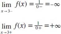
This example can be seen in the accompanying graph.
What is infinitesimal calculus?
Infinitesimal may mean infinitely small in most people’s dictionaries, or bring up thoughts of subatomic particles. To those who study arithmetic, however, it may mean numbers greater in absolute value than zero, yet smaller than any positive real number.
But for those who study calculus, it is an area of mathematics pioneered by Gottfried Leibniz. His idea was based purely on the concept of infinitesimals; this was in opposition to the calculus of Isaac Newton, who based his calculus on the concept of the limit. Although historically the emphasis was placed on the minute, modern infinitesimal calculus actually has little to do with infinitely small quantities.
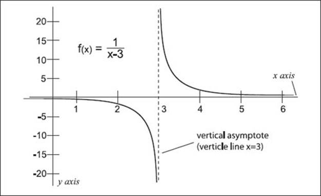
What are vertical asymptotes in association with limits?
Using the example above, as x gets closer to 3, the points on the graph get closer to the vertical line x = 3 (seen as a dashed line on the graph below). This line is called a vertical asymptote. The following charts shows four of the vertical asymptotes for the given function f(x) and their notations.
Graph of an equation with infinity limited by x = 3.
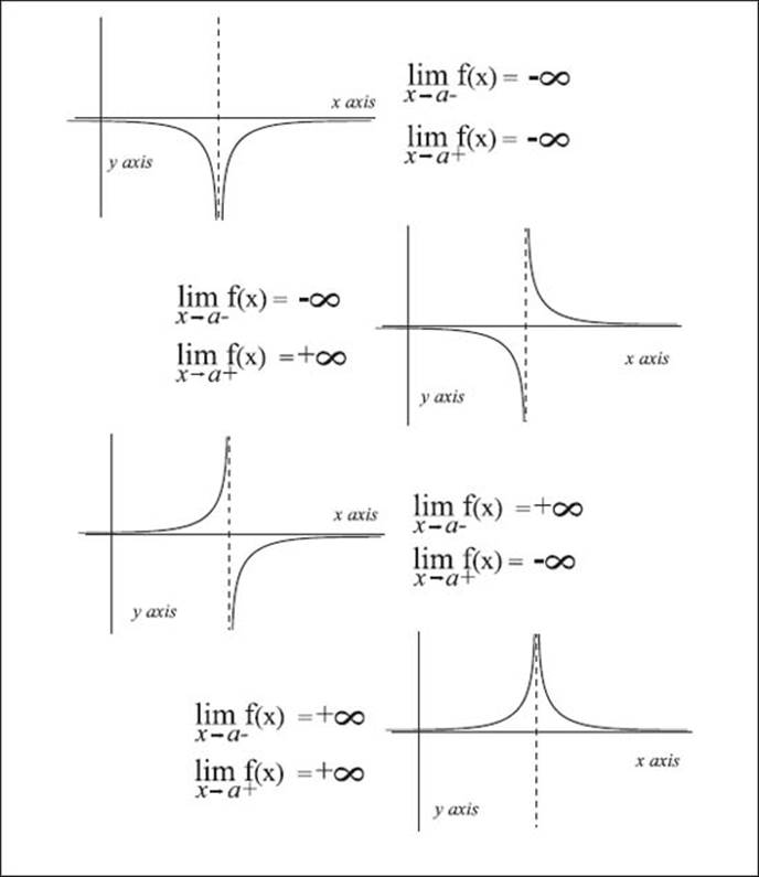
What are horizontal asymptotes in association with limits?
A horizontal asymptote is similar to a vertical asymptote, but it is associated with the y axis. For example, for the function
![]()
gives a solution of:

and, thus, the implied limit is:
![]()
This is because we know that:
![]()
And as x gets larger (or closer to ±∞) the points on the graph come closer to the horizontal line y = 2 (seen as a dashed line on the graph on page 225), which is called the horizontal asymptote.
Four examples of graphed equations limited by vertical asymptotes.
What does continuous and discontinuous mean in calculus?
When talking about polynomial functions, we know that a polynomial function P(x) satisfies the limit function:
![]()
in which a represents all real numbers. This is called continuity.
A graphed equation limited by horizontal asymptote y = 2.
But if f(x) is a function on an interval around a, then f(x) is continuous at a iff (see below for the definition of “iff”):
![]()
if it is not, then f(x) is called discontinuous at a.
What is the concept of bound?
Similar to sequences (see elsewhere in this chapter), in calculus bounds are divided into the upper (either greater than or equal to every other number in a set of numbers; or greater than or equal to all the partial sums of a sequence) or lower (less than or equal to every other number). The symbol for infinity (∞) is used to denote a set of numbers without bound, or that increase or decrease “to infinity.” In calculus, the bounds can be divided even more into greatest or least. For example, the greatest lower bounds and least upper bounds are of special interest to calculus, as those numbers may or may not be found within a set.
What does the strange symbol “iff” mean in calculus?
The symbol (or “word”) iff actually is shorthand for “if and only if.” It is not only mathematics that depends on the iff, but also philosophy, logic, and many technical fields. It is usually italicized; in addition, the phrase “P is necessary and sufficient for Q” is also seen as “Q iff P.” The corresponding logical symbols for “if and only if” are ↔ and ≡.
DIFFERENTIAL CALCULUS
What is the differential calculus?
Differential calculus is the part of “the” calculus that deals with derivatives. It deals with the study of the limit of a quotient, usually written as Δy / Δx, as the denominator (Δx) approaches zero, with x and y as variables.
What is the derivative of a function?
One of the most important, core concepts in modern mathematics and calculus is the derivative of a function—or a function derived from another function. A derivative is also expressed as the limit of Δy / Δx, also said as “the derivative of y with respect to x.” It is actually the rate of change (or slope on a graph) of the original function; the derivative represents an infinitesimal change in the function with respect to the parameters contained within the function.
In particular, the process of finding the derivative of the function y = f(x) is called differentiation. The derivative is most frequently written as dy / dx; it is also expressed in various other ways, including f'(x) (said as the derivative of a function f with respect to x), y’, Df(x), df(x), or Dxy. It is important to note that the differentials, written as dy and dx, represent singular symbols and not the products of the two symbols. Not all derivatives exist for all values of a function; the sharp corner of a graph, in which there is no definite slope—and thus no derivative—is an example.
What is the standard notation for the derivative?
The following represents the definition of the derivative of f(x) (note: in order for the limit to exist, both ![]() and
and ![]() —must exist and be equal; thus, the function must be continuous):
—must exist and be equal; thus, the function must be continuous):
For f (x)’s derivative at point x0:
![]()
For f(x)’s derivative at x = a:
![]()
What is an example of the second derivative?
The second derivative is actually a function’s derivative’s derivative. In other words, the function’s derivative may also have its own derivative, called the second derivative or second order derivative. If we let y = f(x), the second derivative becomes d/dx(dy/dx). This is equal to d2y/dx2, further represented by the symbols f' (x) or y’ One good example of a second order derivative is acceleration—it is actually the second derivative of a change in distance. In other words, the first derivative gives instantaneous velocity (see above) while the second derivative gives acceleration.
Is there a formula for the inverse of a derivative?
Yes. In this case, the derivative of the inverse function represents the inverse of y(x)— or x(y):
![]()
What are the two ways of looking at the derivative?
There are two major ways of looking at the derivative—the geometrical (or the slope of a curve) and the physical (the rate of change). The derivative was historically developed from finding the tangent line to a curve at a point (geometrically); it eventually became the study of the limit of a quotient usually seen as the change in x and y (Δy/Δx). Even today, mathematicians debate which is the best way to describe a derivative.
Geometrically, after determining the slope of a straight line through two points on a graph of a function, and the limit where the change in x approaches zero, the ratio becomes the derivative dy/dx. This represents the slope of a line that touches the curve at a single point—or the tangent line.
Physically, the derivative of y with respect to x describes the rate of change in y for a change in x. The independent variable, in this case x, is often expressed as time. For example, velocity is often expressed in terms of s, the distance traveled, and t, the elapsed time. In terms of average velocity, it can be expressed as Δs/Δt. But for instantaneous velocity, or as Δt gets smaller and smaller, we need to use limits—or the instantaneous velocity at a point B is equal to:
![]()
What are some examples of derivatives of “simple” functions?
The following lists some derivatives of “simple” functions:
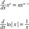
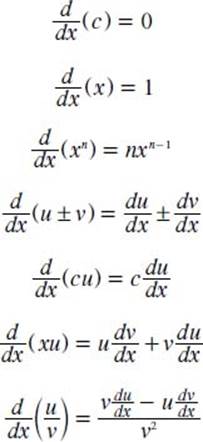
What are some simple derivatives as functions of the variable x?
There are simple derivatives as functions of the variable x. In this case, u and v are functions of the variable x, and n is a constant:
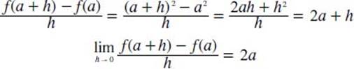
What is an example of computing the derivative?
The following solves the derivative at x = a for the function f(x) = x2, using the definition for a derivative (see above):
What is the Mean-Value Theorem?
The Mean-Value Theorem has nothing to do with crankiness, but it is one of the most important theoretical tools in the calculus. In written terms, it is defined as the following: If f (x) is defined and continuous on the interval [a, b], and differentiable on (a, b), then there is at least one number on the interval (a, b)—or a < c < b—such that:
![]()
When f(a) = f(b), this is a special case called Rolle’s Theorem, when we know that f (c) will equal zero. Interpreting this, we know that there is a point on (a, b) that has a horizontal tangent.
It is also true that the Mean-Value Theorem can be put in terms of slopes. Thus, the last part of the above equation (on the right of the equal sign) represents the slope of a line passing through (a, f(a)) and (b, f(b)). Thus, this theory states that there is a point c ∈ (a, b), such that the tangent line is parallel to a line passing through the two points.
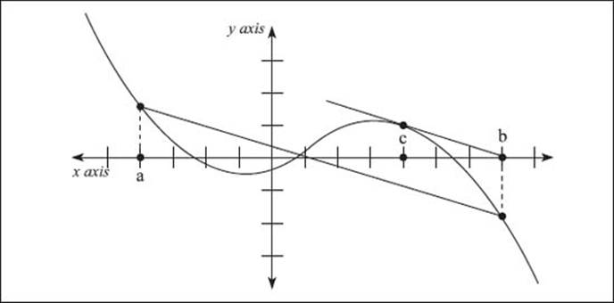
This graph illustrates the concept of the Mean-Value Theorem.
Are there higher derivatives of a function?
Yes, there are higher derivatives of a function, often referred to as higher order derivatives. The “initial” derivative is often written as f' (x), but the “ ' ” is assumed in most cases. The next derivative is the second derivative (second order derivative), most often written as f'' (x); the next is the third derivative, or third order derivative, most often written as f''' (x); fourth derivative, or fourth order derivative, most often written as f(4)(x); and so on. The notation for the higher derivatives, or the nth derivative, is as follows:
![]()
This equation is also seen written as Dn (y) = dny/dxn.
What is a partial derivative?
Partial derivatives (seen written as the symbol δ) are derivatives of a function containing multiple variables that have all but the variable of interest held fixed during the differentiation. Thus, when a function f (x, y, …) depends on more than one variable, the partial derivative can be used to specify the derivative with respect to one or more variables. There are other terms, too: Partial derivatives that involve more than one variable are called mixed partial derivatives. And a differential equation expressing one or more quantities in terms of partial derivatives is called, logically, a partial differential equation. These equations are well known in physics and engineering, and most are notoriously difficult to solve.
What are the product, quotient, power, and chain rules for derivatives?
There are numerous rules for derivatives of certain combinations of functions, including the product, quotient, power, and chain rules. The following lists their common notation:
For a product:
![]()
where f' is the derivative of f with respect to x.
For a quotient:
![]()
where, again, f' is the derivative of f with respect to x.
For a power:
![]()
For a chain:
![]()
Or:
![]()
where ∂z/∂x is a partial derivative.
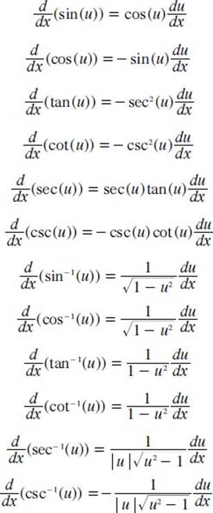
What are the derivatives of trigonometric functions?
There are also derivatives of the six major trigonometric functions—sine, cosine, cotangent, cosecant, tangent, and secant (for more information on these trigonometric functions, see “Geometry and Trigonometry”). The following lists the formulas for those derivatives (in this case, the functions are written with respect to the variable u):
INTEGRAL CALCULUS
What is the integral calculus?
The integral calculus is the part of “the” calculus that deals with integrals—both the integral as the limit of a sum and the integral as the antiderivative of a function (see below for more information). In general, the integral calculus is the limit of a sum of elements in which the number of the elements increase without bound, while the size of the elements diminishes. It is also considered the second most important kind of limit in the calculus (the first being limits in association with derivatives). It was originally developed by using polygons to approximate areas of geometrically shaped objects such as circles.
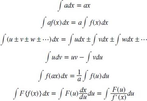
What are some common integrals in the calculus?
There are many standard integrals used in the calculus. The following lists only a few of those integrals in their common form:
What is the definite integral?
In actuality, the area shown on page 233 is actually determined using limits. In the function f(x), as n gets larger, the numbers determined by left (n) and right (n) will get closer and closer to the area Ω. This is seen as the following notation:
![]()
Thus, in the calculus terms, the area of the above graphic region is called the definite integral (also said as “the integral”) of f(x) from a to b, and is denoted by the following notation:
![]()
The variable x can be replaced with any other variable. In other words, if the limits of integration (a and b) are specified, it is called a definite integral, and it can be interpreted as an area or a generalization of an area.
What is the graphic representation of the approximation of an area under a curve using integration?
It’s easier to see the approximate area under a curve using integration by means of graphs—it all has to do with rectangles. The idea is to extend lines from the ends of the curve (here, f(x)) to the x-axis (or y-axis, depending on the curve); we’ll call the total area under the curve Ω, then divide the entire area under the curve into equal-width sections (x1, x2, x3, and so on) that are equal to parts of Ω (the subregions Ω1 Ω2, and so on). The next step is to figure out the area of a rectangle if each section was “cut off” below the curve and then above the curve. This creates rectangles defined by left- and right-end points. From the left- and right-sums, and a few more calculations, we can approximate the area of Ω. This can be seen graphically on the accompanying charts.
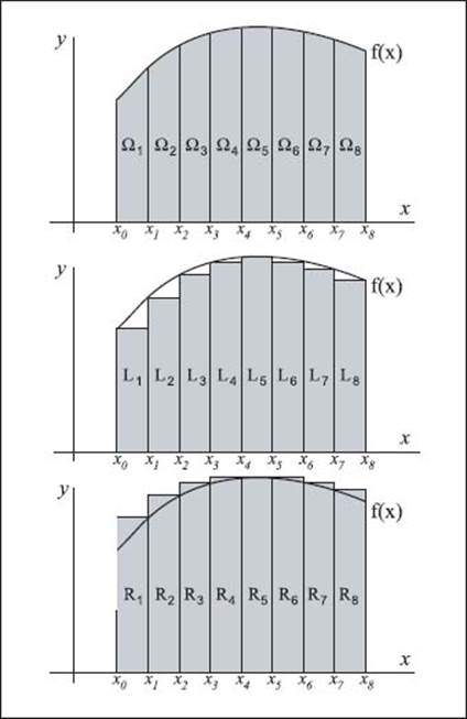
To calculate the area beneath a curve (top), you can first divide the area into equal parts with rectangles both beneath (middle) and above (bottom) the curve. Adjusting the width of the curves will result in an estimate that closely approximates the actual area.
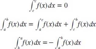
What are some properties of the definite integral?
There are several useful properties of the definite integral. Theorem one is based on the idea that if f(x) and g(x) are defined and continuous on [a, b], except perhaps at a finite number of points, then the following applies in which alpha is a constant:
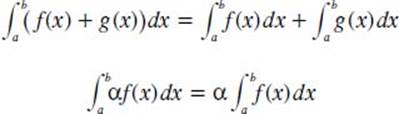
Theorem two is based on the idea that if f(x) is defined and continuous on [a, b], except at a finite number of points, then the following applies for any arbitrary numbers a and b, and any c ∈ [a, b]:
What is an indefinite integral?
From the above, we learned that when the limits of integration (in the case of a and b above) are specified, it is called a definite integral. Contrarily, if no limits are specified, it is called an indefinite integral. Thus, the indefinite integral is most often defined as a function that describes an area under the function’s curve from some undefined point to another arbitrary point. This lack of a specified first point leads to an arbitrary constant (usually denoted as C) that is always part of the indefinite integral.
What are antiderivatives and antidifferentiation?
An antiderivative is often interpreted as the same as an indefinite integral, but they actually do differ in definition. Using the notations below describing the Fundamental Theorem of the Calculus (see boxed text for definition of the Fundamental Theorem of the Calculus), the function F(x) is an antiderivative of f(x), described as also equal to the integral of f(x). The actual process of finding F(x) from f(x) is called integration or antidifferentiation.
What is an improper integral?
An integral as seen above means that the function f(x) needs to be bounded on the interval [a, b] (both real numbers), and the interval also must be bounded. But an improper integral is one in which the function f(x) becomes unbounded (called a type I improper integral) or the interval [a, b] becomes unbounded (a = -∞ or b = +∞, which is called a type II improper integral).
What is the Fundamental Theorem of the Calculus?
The Fundamental Theorem of the Calculus is the connection (or, more accurately, the bridge) between the integral and the derivative; in other words, it is another way of finding the area under a curve (see above) by evaluating the integral. In particular, if F(x) is a function whose derivative is f(x), then the area under the graph of y = f(x) between the points a and b is equal to F(b) - F(a). This is seen as the following notations:
![]()
The number F(b) - F(a) is also denoted by
![]()
Thus,
![]()
Are there double and triple integrals?
Yes, there are double and triple integrals—and even multiple integrals in equations (∫∫, ∫∫∫, and so on). For example, the integration of a function of three variables, w = f(x, y, z), over a three-dimensional region R in xyz-space (three-dimensional space) is called a triple integral. The notation is as follows:
![]()
To compute the iterated integral, we need to integrate with respect to z first, then y, then x. And when we integrate with respect to one variable, all the other variables are assumed to be constant.
DIFFERENTIAL EQUATIONS
What are differential and ordinary differential equations?
Logically, a differential equation is one that contains differentials of a function, with these equations defining the relationship between a function and one or more derivatives of that function. More specifically, differential equations involve dependent variables and their derivatives with respect to the independent variables. To solve such equations means to find a continuous function of the independent variable that, along with its derivatives, satisfies the equation. An ordinary differential equation is one that involves only one independent variable.
What is an example in which differential equations are used?
There are definitely many real-life examples using differential equations; for example, the problem of bacterial growth, which involves quantity and its derivative. Scientists know that bacterial growth depends on how many bacteria exists initially; therefore, if one takes two bacteria, the first increase is by two, then by four, then by eight, and so on. If P (t) is the population (P) of the bacteria at any given time (t), one way to express the rate of change in the number of bacteria over time using differential equations is as follows:
dP / dt
Since it depends on the population P, the equation then becomes:
dP / dt = aP (t)
in which a is a constant that can be used to fit the situation; for example, how long it takes the little critters to reproduce. This is called an equations that relates a certain quantity to it’s derivative—and a classic way of looking at how a differential equation describes exponential growth.
What do the order and degree of a differential equation mean?
The order of a differential equation is simply the highest derivative that appears in the equation. The degree of a differential equation is the power of the highest derivative term. (For more information about power, see “Math Basics.”)
What are implicit and explicit differential equations?
As seen above, an ordinary differential equation is one involving x, y, y', y'', and so on. Now add the idea that the order of the highest derivative is n. Thus, if a differential equation of order n has the form F(x, y', y'', …y(n)) = 0, then it is called an implicit differential equation. If it is of the form F(x, y', y'', … y(n - 1)) = y(n), it is called an explicit differential equation.
What is an example of a differential equation?
An example of a differential equation involves letting y be some function of the independent variable t. Then a differential equation relating y to one or more of its derivatives is as follows:
![]()
In this equation, the first derivative of the function y is equal to the product of t2 and the function y itself. This also implies that the stated relationship holds only for all t for which both the function and its first derivative are defined.
What are some first-order differential equations?
A first-order differential equation is one involving the unknown function y, its derivative y', and the variable x. As seen above, these types of equations are usually referred to as explicit differential equations.
There are several types of first-order differential equations, including separable, Bernoulli, linear, and homogeneous (for explanations of the last two, see below). A first-order differential equation takes the form:
![]()
What is a linear differential equation?
A linear differential equation is a first-order differential equation that has no multiplications among the dependent variables and their derivatives, which means the coefficients are functions of independent variables. Other terms associated with such differential equations are nonlinear differential equations, which have multiplications among the dependent variables and their derivatives, and quasi-linear differential equations, in which a nonlinear differential equation has no multiplications among all the dependent variables and their derivatives in the highest derivative term.
What are the “conditions” in reference to differential equations?
In general, there are two “conditions” when discussing differential equations. The first are called initial conditions, in which constraints are specified at the initial point (usually in reference to time); such problems are called initial value problems. The other condition is the boundary condition, in which constraints are specified this time at the boundary points (usually in reference to space), with such problems called boundary value problems.
What are the “solutions” relative to differential equations?
There are three types of “solutions” when discussing differential equations:
General solution—This includes the solutions obtained from integration of the differential equations. In particular, the general solution of an nth order ordinary differential equation has n arbitrary constants from integrating n times.
Singular solution—Solutions that can’t be expressed by the general solutions. Particular solution—Solutions obtained from giving specific values to the arbitrary constants in the general solution.
What techniques are used to solve first-order differential equations?
There are usually three major ways to solve first-order differential equations: analytically, qualitatively, and numerically. The analytical way includes the examples mentioned above, such as the linear and separable equations. Qualitative methods include such methods as defining the slope of a field of a differential equation. Finally, numerical techniques can be thought of as something close to Euler’s method, a way of finding the largest divisor of two numbers.
What is Euler’s method?
Swiss mathematician Leonhard Euler (1707–1783) was one of the most prolific mathematicians who ever lived. He developed Euler’s method, which is a way of determining the largest divisor of two numbers. For example, if we want to find the largest divisor of the numbers 6,975 and 525, we consider one to be the large number and the other the small number. We already know both numbers are divisible by 0 and 5 (as they both end in 5), but how do we determine if they have a larger divisor? And if so, what is that number?
The key is to take the remainders of long division until we arrive at a remainder of zero. In this instance, we would first divide 6,975 by 525; the answer comes out to 13 and a remainder:
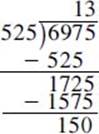
Take the remainder—in this case, 150—and then divide it into the 525. Take that remainder (which turns out to be 75) and divide it into the 150 remainder. The next iteration leads to no remainder (zero).
|
Large Number |
Small Number |
Remainder |
|
6975 |
525 |
150 |
|
525 |
150 |
75 |
|
150 |
75 |
0 |
Thus, taking the number before we reached the zero—or 75—gives us the largest common divisor of both 6,975 and 525.
What are first-order homogeneous and non-homogeneous linear differential equations?
These differential equations may be long-winded phrases, but they are actually types of first-order differential equations. A first-order homogeneous linear differential equation can be written in the notation as follows:
![]()
The first-order homogeneous linear differential equations are those that place all terms that include the unknown equation and its derivative on the left-hand side of the equation; on the right-hand side, it is set equal to zero for all t.
The non-homogeneous linear differential equations are those that, after isolating the linear terms containing y(t) and the partial differentials inside the above large parentheses on the left side of the equation, do not set the right-hand side identically to zero. It is often represented by one function, such as the b(t) (see below). The standard notation is as follows:
![]()
What are systems of differential equations?
In real-life situations, quantities and their rate of change depend on more than one variable. For example, the rabbit population, though it may be represented by a single number, depends on the size of predator populations and the availability of food. In order to represent and study such complicated problems we need to use more than one dependent variable and more than one equation. Systems of differential equations are the tools to use. As with the first-order differential equations, the techniques for studying systems fall into the following three categories: analytic, qualitative, and numeric.
What is a nonlinear differential equation?
From above, we know that linear equations have specific rules; for example, the unknowns y, y', and so on, will never be raised to a power more than 1; they will not be in the denominator of a fraction; y times y' is never allowed (because two unknowns multiplied together is, in a sense, a power 2 of unknowns); and they won’t be inside another function (such as a sine).
But a nonlinear equation is much different, allowing for powers of 2(y' = y2), multiplying differences (y × y' = x); and even being inside another function (y' = x sin y).

Rabbit populations are affected not only by birth rates, but also by factors such as predation, disease, and available food supplies. Systems of differential equations may be used to take all these elements into consideration and estimate actual population numbers.
Thus, the nonlinear equations are not as easy to solve as linear differential equations. But that does not mean they lack importance. In fact, because nonlinear equations are more realistic in describing real-life problems, they are much more interesting (and challenging) to mathematical and scientific researchers in many fields.
VECTOR AND OTHER ANALYSES
What is a vector?
A vector is considered to be an element of a linear or vector space. A vector is different than a point, as it represents the displacement between two points, not the physical location of a point in space. Vectors also define a direction; points do not. Vectors are usually represented by a line segment in a specific direction on a graph, with an arrow at one end of the segment. They can also be represented in several ways, including bold letters in an equation, for example, vectors A and B, and with arrows above the vector, such as ![]() .
.
What is the component of a vector?
A component of a vector is one with n numbers in a certain order. It is usually listed as (x1, x2, …, xn), in which the numbers within the parentheses are called the components of the vector ![]() .
.
Logically, an infinite number of vectors can have the same components. For example, if the components are [3, 4], we know there are an infinite number of pairs of points in the plane with x and y coordinates whose respective differences are 3 and 4. All these vectors are parallel to each other, equal, and have the same magnitude and direction. Therefore, any vector with components of a and b can be said to be equal to the vector [a, b].
How is the magnitude of a vector determined?
The magnitude of a vector is equivalent to the length of a vector. Placing a pair of vertical lines (similar to the absolute value symbol) around a vector implies the magnitude of the vector. For example, if the variable V is used to represent a vector, then the expression ![]() indicates the magnitude of the vector.
indicates the magnitude of the vector.
What do columns and rows mean when discussing vectors?
Vectors can be described by columns and rows. For example, two-dimensional and three-dimensional vectors are usually represented as a single vertical column of numeric values. The following lists such columns in two and three dimensions:
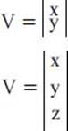
A row vector is usually used for problem solving in which a vector is described as V = (x, y, z) during the specification of a problem. But note: Row vectors should not really be used with any mathematical descriptions.
How is the length of a vector calculated?
The length of a vector is calculated by taking the square root of the sum of the squares of each coordinate. For example, if the vector is defined by (x, y, z), then the length (L) of the vector is calculated this way:
![]()
What is a normalized vector?
A normalized (or unit) vector is one in which the sum of the squares of all coordinates is equal to one. For example, the vector (2, 2, 0) is not normalized; the vectors (0.707, 0.707, 0.0) and (1.0, 0.0, 0.0) are normalized. (An outward normal is another name for a normalized vector; it represents the direction that a polygon surface or vertex [end-point] is facing.) Normalized (or unit) vectors are often seen written as ![]() , but more usually as
, but more usually as ![]() (the
(the ![]() is often referred to as a “hat”).
is often referred to as a “hat”).
A vector can be normalized by calculating the magnitude or length of the vector and dividing each coordinate by this value. For example, consider the following vector:

How are vectors used?
Many physical quantities—especially those in association with mathematics and science—can be represented by vectors, such as force, velocity, and momentum. In specifying these quantities, one must state not only how large it is but also in what direction it acts. Even more complex is the use of multidimensional vectors for such problems as relativity, wind velocities in an atmosphere, and in determining electromagnetic fields.
The length of this vector is 5.0 (see above to determine how to solve for length of the vector); or |V| = 5.0. Thus, the value of the normalized vector is given by:
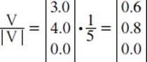
In this case, 0.6 squared equals 0.36; 0.8 squared equals 0.64. Both added together with the zero equals 1. (If the vector is already normalized, then the value of |V| will be equal to one, and after division the vector will remain as it was before.)
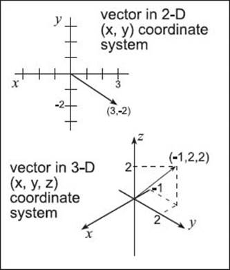
How can vectors be represented in various dimensional space?
Vectors can be found in two-, three-, or multi-dimensional space. Two-dimensional vectors are seen visually on a graph as a line with an arrow connecting two points. A two dimensional vector is defined by length and direction measured by the angles that the arrow makes with the x and y coordinate system axes; a vector in such a coordinate system is written as two components, (x, y).
Vectors in a three-dimensional space are represented with three numbers, one along each coordinate axis. These are the coordinates of the arrow point, usually as (x, y, z) if the arrow starts at the origin. A more complex vector is one with multiple components, in which several different numbers in ordered n-tuples represent a vector. For example, (4, 1, -2, 0) is an ordered 4-tuple representing a vector in four dimensions.
What is a polar coordinate system?
In effect, a polar coordinate system “wraps” a two-dimensional (Euclidean) coordinate system onto the surface of a sphere (for more information about coordinate systems, see “Geometry and Trigonometry”). A polar coordinate system examines a point in space defined in terms of its position and distance on a sphere with a unit radius. The center of the sphere is considered the origin; the first two coordinates are the longitude and latitude on the sphere; the third coordinate defines the distance of the point from the center of the sphere—the values of latitude, longitude, and height. In polar coordinates—it’s easy to see on a globe of our own planet—latitude ranges from +90 to -90, longitude ranges from -180 to +180, and height ranges from zero to infinity. Height can also be negative: The North Pole is at coordinates of (+90, —, +r) (the “—” means there is no longitude), the South Pole is at coordinates of (-90, —, -r), and a point on the equator is at coordinates (0, 0, r).
How are vectors added?
One way to combine vectors is through addition (or composition). This can be done algebraically or graphically. For example, to add the two vectors U [-3, 1] and V [5, 2], one can add their corresponding components to find the resultant vector R [2, 3]. One also can graph U and V on a set of coordinate axes, completing the parallelogram formed with U and V as adjacent sides, obtaining R as the diagonal from the common vertex of U and V.
How is the product of two vectors determined?
There are two distinct types of products of two vectors: scalar and vector products, sometimes called the inner and outer products (mostly in reference to tensor products; see below). The scalar (or dot) product of two vectors is not a vector because the product has a magnitude but not a direction. For example, if A and B are vectors (of magnitude A and B, respectively), their scalar product is: A • B = AB cos θ, in which θ is the angle between the two vectors. This scalar quantity is also called the dot product of the vectors. These equations obey the commutative and distributive laws of algebra (for more information, see “Algebra”). Thus, A • B = B • A; A • (B + C) = A • B + A • C. If Ais perpendicular to B, then A • B = 0.
The vector (or cross or skew) product of A and B is the length C = AB sin θ; its direction is perpendicular to the plane determined by A and B. In this case, this kind of multiplication does not follow the commutative law, as A • B = -B • A.
What is vector analysis?
Vector analysis is the calculus of functions with variables as vectors—a part of calculus also known for its derivative and integral equations. The components of a vector do not always have to be constants. They can also be variables and functions of variables, such as the position of a body moving through space represented by a vector whose x, y, and z components are all functions of time. In this case, the calculus can be used to solve such vector functions, which are also called vector analysis.
What is a linear combination?
Alinear combination is a combination or the sum of two or more entities with each multiplied by some number (with not all the numbers being zero). Linear combinations of vectors, equations, and functions are common. For example, if x and y are vectors and a and b are numbers, then ax + by is a linear combination. (For more information about equations and functions, see “Math Basics” and “Algebra.”)
What are some other types of analysis?
There are numerous other analyses in mathematics and the sciences besides vector analysis. And each one has applications that sometimes intermingle but most often has specific uses in certain areas—from computer programming to electronics.
At one time, the study of tensors was known as the absolute differential calculus, but today it is simply called tensor analysis. Tensors were originally invented as the extensions of vectors. Tensor analysis is concerned with relations or laws that remain valid regardless of the coordinate system used to specify the quantities.
Complex analysis (or complex variable analysis) is the study of complex numbers and their derivatives, mathematical manipulations, and other properties. It is mostly used to find the solution to holomorphic functions, or those that are found in a complex plane, use complex values, and are differentiable as complex functions. Complex variables deal with the calculus of functions of a complex variable, incorporating differential equations and complex numbers; for example, one such variable of the form z = x + iy, in which x and y are real and the imaginary number i = -1. Complex-variable techniques have a great many uses in applied areas, such as electromagnetics.
Functional analysis is concerned with infinite-dimensional vector spaces and the mapping between them. It is also considered the study of spaces of functions.
There is also differential geometry, truly a branch of geometry, which includes the concepts of the calculus as applied to curves, surfaces, and other geometry entities. Originally, it included the use of coordinate geometry; more recently, it has been applied to other areas of geometry, such as projective geometry. In particular, differential geometry uses techniques of differential calculus to determine the geometric properties of manifolds (a topological space that resembles Euclidean space, but is not).
Another type of analysis is nonstandard analysis, developed in the 1960s, in which hyperreal numbers are used to define the existence of “genuine infinitesimals.” (These are numbers less than one half, one third, one fourth, and so on, but greater than 0.) It is used in several fields, including probability theory and mathematical physics.
What is a tensor?
A tensor is a quantity that depends linearly on many vector variables. They are considered to be a set of n' components that are functions of the coordinates at any point in n dimensional space. Tensors are used in several fields of mathematics, such as the theory of elasticity (stress and strain) and mathematical physics, especially with regard to the theory of relativity.