The Handy Math Answer Book, Second Edition (2012)

APPLIED MATHEMATICS

APPLIED
MATHEMATICS BASICS

What is applied mathematics?

Applied mathematics is not only concerned with using rigorous mathematical methods, but also applications of those methods. It entails a wide range of research in the worlds of biology, computer science, sociology, engineering, physical science, and many other fields, especially in the experimental sciences. In each case, applied mathematics is used by a researcher to more thoroughly understand a particular application or physical phenomena. The many uses of applied mathematics include numerical analysis, linear programming, mathematical modeling and simulation, the mathematics of engineering, mathematical biology, game theory, probability theory, mathematical statistics, financial mathematics, and even cryptography.

How did applied mathematics grow over time?

Historically speaking, applied mathematics was always concerned with using mathematics to solve problems in physics, chemistry, medicine, engineering, the physical sciences, technology, and biology. In fact, applied mathematics is older than pure mathematics, as it was used in areas that formed the core of early physics research, such as mechanics, fluid dynamics, and optics. As mathematical tools became more powerful, these areas of physics became more mathematically based. This mathematical analysis tie to science and engineering has always had a great place in history and has led to some of its greatest discoveries.

Why is there such a demand for applied mathematics in processing of images?

The field of image processing has grown immensely in the past few decades. There is a great demand for an increase in efficient processing of images, especially for multimedia, biology, and medicine, such as enhancing the quality of electron microscope and MRI (Magnetic Resonance Imaging) images. In addition, there is also a great need to develop ways to store more and more information, and especially how to transmit and process the information using computers and networks.

All of these things require the use of several mathematical techniques. Overall, there is no one mathematical theory of image processing. Instead, mathematicians and scientists use several areas of mathematics, including applied, partial differential equations, statistics, etc. to solve image processing needs. As computers and processing becomes even more powerful, these mathematical tools will become even more important.

How has applied mathematics changed over the past few decades?

In the past few decades, applied mathematics has made tremendous strides in explaining our world. In particular, with the advent of more powerful computers and their mathematically driven software—from linked computers over a network to supercomputers—many disciplines that use applied mathematics have greatly advanced. For example, the use of giant wind tunnels to examine wind flow over aircraft only a few decades ago has been replaced by computer simulation. Now the design and testing of aircraft is accomplished by these simulations, making the expense of building physical prototypes a thing of the past because it is now merely a matter of mathematically “drawing” the aircraft on the computer in order to test new designs.

How do various disciplines use applied mathematics?

Depending on the discipline, researchers use applied mathematics in various ways. For example, some disciplines rely heavily on pure mathematics. Numerical analysis—a form of applied mathematics—is a field that uses pure mathematics to decipher partial differential equations and variational methods (for more information about numerical analysis, see below; for partial differential equations, see “Mathematical Analysis”). There are also areas of applied mathematics that overlap other fields of study. For example, there are mathematicians who use applied mathematics to study the structure of matter—especially the behavior of subatomic particles—a field that also overlaps the same types of studies done by subatomic physicists.

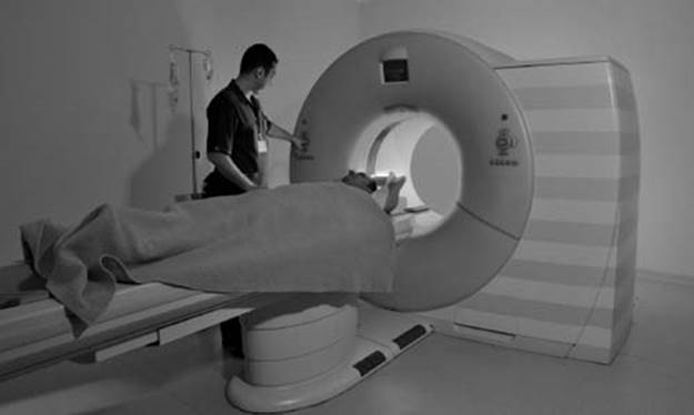
Applied mathematics is used in high-tech image processing, such as with this MRI (Magnetic Resonance Imaginge) machine used in hospitals to create scans of the inside of patients’ bodies.

Why has the combination of mathematical analysis methods and computers been so important?

The combination of mathematical analysis and computers has been a strong alliance, especially with regard to engineering, technology, and the sciences. In the past few decades, researchers have used this combination to help predict the weather, describe in great detail nuclear fusion in the Sun, understand the movement of space bodies around the solar system (orbital mechanics), and the flow of water in underground aquifers (fluid dynamics). There are also the studies of chaos—the unpredictable behavior of nonlinear systems—and quantum mechanics, or the physics of very small particles, both of which entail the use of applied mathematics and computers.

In addition, in engineering (and almost all technology) the mathematical analysis-computer combination has helped create structures that surround us every day. This includes familiar modes of transportation and communication: from plans for airplanes and bridge construction to designing fiber optic cables and cell phone towers. It also includes how engineers design control systems, which are used in such diverse areas as robotics, aerospace engineering, and biomedical research.

Computers and mathematical analysis have also been a boon to such interdisciplinary fields at operations research (also called decision or management science). In this case, the mathematical science focuses on the effective use of the technology of an organization, such as forecasting, financial engineering, logistics, and industrial engineering. Applications may include, for example, scheduling airplanes and crews; signal processing, such as the transmission of radio signals or traffic light control signals; or managing the flow of water from a reservoir or dam site.

One of many practical applications for mathematics includes processing images, which enhances the ability of electron microscopes like this one to produce more detailed visual information.

PROBABILITY THEORY

What are events and probability?

Probability is a branch of mathematics that assigns a number measuring the “chance” that some “event”—or any collection of outcomes of an experiment—will occur. It is a quantitative description of the likely occurrence of the event, conventionally expressed on a scale from 0 to 1. For example, a very common occurrence has a probability of close to 1; an event that is more rare will have a probability close to 0. In more common usage, the word “probability” means the chance that a particular event (or set of events) will occur—all on a linear scale expressed as a percentage between 0 and 100 percent (%). An even more detailed way of looking at probability includes the possible outcomes of a given event along with the outcomes’ relative likelihoods and distributions.

What is subjective probability?

As the word implies, a subjective probability is thought of as a personal degree of belief that a particular event will occur. An individual’s personal judgment is not based on any precise computation, but is most often a reasonable assessment of what will happen by a knowledgeable person. This is usually expressed on a scale of 0 to 1, or on the percentage scale. For example, if a person’s baseball team has a winning streak, they might believe that their team has a probability of 0.9 of winning the division championship for the year. More likely, they will say their team has a 90 percent chance of winning, not because of any mathematical formula, but only because the team has had a winning record during the year.

What is a sample space?

In any experiment, there are certain possible outcomes; the set of all possible outcomes is called the sample space of the experiment. Each possible result is represented by one and only one point in the sample space, which is usually denoted by the letter S. To each element of the sample space (or to each possible outcome) a probability measure between 0 and 1 is assigned, with the sum of all the probability measures in the sample space equal to 1.

What are ratios and proportions?

A ratio is the comparison of two numbers; it is most often written as a fraction or with a “:”, as in 3/4 or 3:4 to separate the two numbers. For example, if we want to know the ratio of dogs in a shelter that houses 24 animals to the total count, we first determine the number of dogs (say, 10); then the ratio of dogs to animals in the shelter becomes 10/24, or 10:24, which is also said as “10 to 24.” But there are rules to ratios. For example, order matters when talking about ratios; therefore, the ratio 7:1 is not the same as 1:7.

A proportion is an equation with a ratio on each side, and is a statement that two ratios are equal. For example, ½ = 4/8, or ½ is proportional to 4/8. In order to “solve the proportion”—or when one of the four numbers in a proportion is unknown—we need to use cross products to find the unknown number. For example, to solve for x in the following: 1/4 = x/8; using cross product, 4x = 1 × 8; thus, x = 2.

What are some simple probability events?

The probability measure of an event is sometimes defined as the ratios between the number of outcomes. There are many simple illustrations of probability events, many of which we are all familiar with. One of the simplest examples of probability is tossing a coin, with a sample space of two outcomes: heads or tails. If a coin were completely symmetrical, the outcome would more likely be 0.5 (ratio of ½) for heads and 0.5 for tails. As we all know, it never comes out that way, which may or may not mean our coins are not in perfect balance.

What is the probability of drawing a diamond card or an ace from a pack of 52 playing cards?

The probability of drawing a diamond-faced card from a pack of 52 playing cards is easy to determine. Since there are 13 diamond-faced cards in the deck, the probability becomes 13/52 = 1/4 = 0.25.

The probability of drawing an ace from a pack of 52 playing cards is also easy to determine. There are 4 aces in the deck of 52 cards; thus, the probability becomes 4/52 = 1/13 = 0.076923. This represents a much lower probability than drawing a card in a specific suit, illustrated in the preceding example.

Another example is weather records. Many of us keep track of weather over the years. But if one were to gather all the records for the day of May 10 over 30 years from the weather service, one could do some simple probability event measurements. For example, take a (fictitious) sampling of the cloud-covered days in a certain area for the last 30 years on May 10. Say there were 10 cloud-covered May 10s in 30 years; thus, the probability measure would be a ratio of 10/30 to the event that the day will be cloudy on May 10.

Insurance tables are also figured out in a similar way. For example, if, out of a certain group of 1,000 persons who were 25 years old in 1900, 150 of them lived to be 65, then the ratio 150/1,000 is assigned as the probability that a 25-year-old person will live to be 65. On the other hand, the probability of such a person not living to be 65 is 850/1,000 (because the sum of the two measures must be equal to 1). It is true that such a probability statement is valid only for a set group of people, but insurance companies get around this by using a much larger population sample and constantly revising the figures as new data are obtained. Thus, even though many people question the validity of such “broadbrush” results, the insurance companies believe that, probability-wise, the values they use are valid for most large groups of people and under most conditions of life.

How are probabilities of compound events determined?

Besides the probability of simple events, probabilities of compound events can also be computed. For example, if x and y represent two independent events, the probability that both x and y will occur is given by the product of their separate probabilities; and the probability that either of the two events will occur is given by the sum of their separate probabilities minus the probability that both will occur. For example, if the probability that a certain man will live to be 70 is 0.5, and the probability that his wife will live to be 70 is 0.6, the probability that they will both live to be 70 is 0.5 × 0.6 = 0.3; the probability that either the husband or wife will reach 70 is 0.5 + 0.6 - 0.3 = 0.8.

The probability of drawing a particular suit from a pack of cards is 25 percent.

What are the definitions of chance?

Chance is defined in many ways. For example, chance means opportunity to some, or the chance to do something. Chance can also mean luck or fortune, such as running into someone one has not seen in years by “pure chance.” Chance also involves taking a risk, which may include some type of danger.

Mathematically speaking, chance is a measure of how likely it is that an event will occur—in other words, a probability. For example, if a meteorologist says that a hurricane on a certain path has struck the coast of Florida, say, about 4 times out of 10, then the ratio becomes 4 to 10, with the chance of striking under the very same conditions being 40 percent. (In reality, this probability example is too simple; that’s because there are so many variables that affect the movement of the hurricane, including the atmosphere and landmasses.)

What do the terms random and stochastic mean in probability?

When speaking about probability, the term random means the outcomes of an experiment have the same probability of occurring. Because of this, the outcome of the experiment produces a random sample.

Random also is commonly thought of as being synonymous with stochastic, which is from the Greek word meaning “pertaining to chance.” It is usually used to indicate a particular subject seen from the point of view of randomness. Stochastic is often thought of as the “opposite” of deterministic, a term that means random phenomena are not involved. In the case of modeling, stochastic models are based on random trials, while deterministic models always produce the same output for a given starting condition.

Are “random” numbers generated by a computer truly random?

For most general purposes, random numbers generated by a computer can be considered “random.” But in reality, because a computer follows a set of rules in any program, the numbers generated are not truly random. In order for a sequence or specific numbers to be truly random, they must not follow any sort of rules. That’s something to think about the next time you purchase a computer-generated, “random-numbers” lottery ticket.

What is the concept of relative frequency?

Relative frequency is actually another term for proportion. It can be found by dividing the number of times an event occurs by the total number of times the experiment is done. In probability, this is often written in the notation rfn(E) = r/n, in which E is the event, n is the number of times the experiment is repeated, and r is the number of times E occurs. For example, a symmetrical coin can be tossed 50 times (n) in order to find out how many times tails will occur (E). If the result is 20 tails (r) and 30 heads, then the equation becomes 20/50, or 2/5 = 0.4; or, the relative frequency is 0.4 for tails. If this experiment is repeated over and over, the relative frequency will eventually get closer and closer to 0.5, which is the true value that should result when tossing a two-sided symmetrical coin.

How are the terms outcome, sample space, and event related?

These terms are definitely related: The outcome is the result of an experiment or other type of situation involving uncertainty; and the set of all possible outcomes is a sample space. Just as important are events, which are collections of the outcomes of an experiment, or any subset of the sample space. If there is only one single outcome in the sample space, it is called an elementary or simple event; events with more than one outcome are called compound events.

What are independent events in probability?

In probability theory, events are independent if the probability that they occur is equal to the product (multiply together) of the probabilities of either two or more individual events. (This is also often called statistical independence.) In addition, the occurrence of one of the events can give no information about whether or not the other event(s) will occur; that is, the events have no influence on each other.

For example, two events, A and B, are independent if the probability of both occurring equals the product of their probabilities, or P (A) | P(B) (the symbol “|” is often used to depict the product of the events in probability theory). One good example involves playing cards. If we wanted to know the probability of two people each drawing a king of diamonds (two independent events), it would be defined as A = 1/52 (the probability that one person will draw a king of diamonds) and B = 1/52 (the probability that the other person will draw a king of diamonds, assuming the first person puts the first drawn card back into the deck). Substituting the numbers into the equation, the result is: 1/52 | 1/52 = 0.00037, or a slight chance that both people will draw the king of diamonds from the deck.

What is conditional probability?

Conditional probability is often phrased as “event A occurs given that event B has occurred.” The common notation is a vertical line, or A | B (said as “A given B”). Thus, P (A | B) denotes the probability that event A will occur given that event B has occurred already.

Since there is always room for improvement—even in probability—conditional probability incorporates the idea that once more information becomes available, the probability of further outcomes can be revised. For example, if a person brings a car in for an oil change every 3,000 miles, it can be calculated that there is a probability of 0.9 that the service on the car will be completed within two hours. But if the car is brought in during a seatbelt recall, the probability of getting the car back in two hours might be reduced to 0.6. This is the conditional probability of getting the car back in two hours if there is a seatbelt recall taking place.

What is Bayes’s theorem?

Bayes’s theorem is a result that lets new information be used to update the conditional probability of an event. The theorem was first derived by English mathematician Thomas Bayes (1702–1761), who developed the concept to use in situations in which probability can’t be directly calculated. The theorem gives the probability that a certain event has caused an observed outcome by using estimates for all possible outcomes. Its simplest notation is as follows:

What are mutually exclusive events?

Mutually exclusive events are those that are impossible to occur together. For example, a subject in a study of male and female humans can’t be both male and female. Males are males; females are females. Thus, depending on what the study is about (such as a study of how many males versus females go to college from a certain high school), both “events” will be mutually exclusive.

What are the addition rules of probability?

In probability theory, the addition rule is used to determine the probability of events A or B occurring. The notation is most commonly seen in terms of sets: P(A∪B) = P(A) + P(B) - P(A∩B), in which P(A) represents the probability that event A will occur, P(B) represents the probability that event B will occur, and P(A∪B) is translated as the probability that event A or event B will occur. For example, if we wanted to find the probability of drawing a queen (A)or a diamond (B) from a card deck in a single draw, and since we know there are 4 queens and 13 diamond cards in the deck of 52, the equation and resulting probability becomes: 4/52 + 13/52 - 1/52 = 16/52 (the 1/52 is derived by multiplying 4/52 × 13/52).

But there are also rules of addition for mutually exclusive and independent events. For mutually exclusive events, or events that can’t occur together, the addition rule reduces to P(A∪B) = P(A) + P(B). For independent events, or those that have no influence on each other, the addition rule reduces to P(A∪B) = P(A) + P(B) - P(A) | P(B).

What are the multiplication rules of probability?

In probability theory, the multiplication rule is used to determine the probability that two events, A and B, both occur. As with the addition rules, the notation for multiplication rules of probability are most commonly seen in terms of sets: P(A∩B) = P(A|B) • P(B) or P(A∩B) = P(B|A) • P(A), in which P(A) represents the probability that event A will occur, P(B) represents the probability that event B will occur, and P (A∩B) is translated as the probability that event A and event B will both occur. In addition, P(A|B) is the conditional probability that event A occurs given that event B has already occurred, and P(B A) is the conditional probability that event B occurs given that event A has already occurred. Similar to the addition rules, if there are independent events (or those that have no influence on one another), the equation reduces to P(A∩B) = P(A) • P(B).

What is the law of total probability?

The law of total probability can be written as follows: The probability that an event A will occur, P(A), is equal to the probability that event A and event B both occur, plus the probability that event A and event B' occur (or A occurs and B does not). Using the multiplication rule, this is written as:

What was the “gambler’s ruin”?

The gambler’s ruin is an application of the law of total probability that was first proposed by Dutch mathematician and astronomer Christiaan Huygens (1629–1695), although many people before him, including astronomer Galileo Galilei (1564–1642), brought up the same probability problem, but phrased it differently. By 1656, Huygens wrote a draft version of Van Rekeningh in Spelen van Geluck, a treatise about fifteen pages long based on what he heard about the correspondence of French scientist and religious philosopher Blaise Pascal (1623–1662) and French mathematician Pierre de Fermat (1601–1665) the previous year. Of the fourteen problems he presents, the last five became known as the “gambler’s ruin.”

How is set theory used to represent the relationships among events?

Statisticians often use the set theory to represent relationships among events (collections of outcomes of an experiment). This is usually written in the following notation, in which A and B are two events in the sample space S:

· A∪B, or “either A or B occurs, or both”; this is said as “A union B” in set theory;

· A∩B, or “both A and B occur”; this is said as “A intersection B” in set theory;

· A⊆B, or “if A occurs, so does B occur”; this is said as “A is a subset of B” in set theory;

· A’, or “A does not occur.”

In particular, Huygens (and others) wanted to find the probability of a gambler’s ruin. A common way of expressing the idea is by a game that has two players, with the game giving a probability q of winning one dollar and a probability (1 - q) of losing one dollar. In the problem, if a player begins with 10 dollars and intends to play the game repeatedly until he either goes broke or increases his holdings to 20 dollars, the question asked is: “What is his probability of going broke?” The answer involves quite a bit of probability computation. (For more information about the gambler’s ruin, see “Recreational Math.”)

What are permutations, combinations, and repeatables?

In order to perform certain probability problems, specific counting techniques need to be used, including determining the number of permutations, combinations, or repeatables. The following explains each term; the examples are based on a set of five cats on a shelf—a, b, c, d, and e, for convenience. (Note: The cats can be arranged in 120 ways, expressed as 5 × 4 × 3 × 2 × 1 = 5! [“5 factorial”] = 120).

The number of permutations is the number of different ways specific entities within the cat group can be arranged, with the positions being important. For example, given five cats, how many unique ways can they be placed in three positions on the shelf if position is important? The answers include ade, aed, dea, dae, ead, eda, abc, acb, bca, bac, etc.—a total of 60 ways. The notation for this is 5 P3 = 5!/(5 - 3)! = 5 × 4 × 3 × 2 × 1 / (2 × 1) = 5 × 4 × 3 = 60 (P in this case stands for permutations).

Dutch mathematician and astronomer Christiaan Huygens devised the notion of the “gambler’s ruin.”

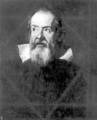
Galileo Galilei, best known for his work as an astronomer, had already discovered the ideas of probability later restated as the “gambler’s ruin” by Christiaan Huygens.

Combinations mean the number of different ways specific entities can be grouped; but in this case, position does not matter. For example, in the problem of the cats, how many can be grouped into threes if position does not matter? The answers include abc, abd, abe, acd, ace, ade; but groupings such as cba are not allowed since it is equal to another combination: abc. The notation for this is 5 C3 = 5!/((5–3)! × 3!) = 5 × 4 × 3 × 2 × 1/(2 × 1 × 3 × 2 × 1) = 5 × 2 = 10 (C in this case stands for combinations).

With repeatables, position is important, too. But in this case, if one has five different cats, and many clones of each, how many unique ways can they be placed in three positions? This answer includes aaa, bbb, ccc, ddd, eee, eec, cee, etc.—a total of 125 ways. The notation for this is 5 R3 = 5³ = 125 (R in this case stands for repeatables).

What is the Markov model?

The Markov model was first developed by Russian mathematician Andrey (Andrei) Andreyevich Markov (1856–1922) about a century ago. It is a statistical method that estimates the likelihood of a future event based on patterns observed in the past. They are most useful when a decision problem involves risk that is continuous over time, when the timing of events is important, and when important events may happen more than once.

The Markov chain also has applications in statistical models, and is a mathematical system that undergoes transitions from one state to another in a chainlike manner.

Most often today, it is used in such fields as economics, genetics, and computer speech-recognition. It is often used extensively in clinical medical studies; for example, Markov models assume that a patient is always in one of a finite number of discrete health states, called Markov states. Such studies can be evaluated by matrix algebra or as a Monte Carlo simulation.

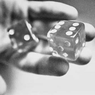
Games such as coin tossing and dice rolling are common examples of the rules of probability in action.

What are some examples in which probability is used?

There are thousands of examples in which probability is used, some are familiar, and some originate from the seamier side of life. For example, everyone has played at coin tossing at one time or another. Although there is no such thing as an idealized coin— a circular one of zero thickness—most coin tosses use the coins available, with either side face up (“heads” or “tails”; also phrased “heads up/down” or “tails up/down”). Thus, one can think of a coin as a two-sided die in lieu of the six-sided cubes we are all used to in a game of dice. If a coin is tossed with a good amount of spin, we can denote the two possible results as H for heads and T for tails. If we repeat the tosses N number of times, we obtain N(H) heads and N(T) tails. Thus, the fraction of N(H)/N and N(T)/N can be thought of as the chance (probability) to get a head or tail, respectively; P(H) and P(T) are the most common notations that represent the probability to get heads and tails, respectively. If we toss the coin many, many times, the result should be close to 0.5. Of course, this means that if we bet on the chances of heads and tails, we will not be much of a winner if we play too many games—and we will have to have really good luck to win if we play fewer games.

What is a random walk?

Although one might think of a random walk as one that a person takes on the spur of the moment in a part of town he has never walked before, it actually means something totally different in probability theory. A random walk is a random process made up of a discrete sequence of steps, all of a fixed length. For example, in physics, the collisions of molecules in a gas are considered a random walk responsible for diffusion; also in physics, random walks and some of the self-interacting walks are found in quantum field theory. In economics, the “random walk hypothesis” is used to understand and model stock share prices, along with other factors. Biologists use random walks to understand individual animal movements; and geneticists who study population use a random walk to describe the statistical properties of genetic drift. One of the more understandable random walks is familiar to most of us—it is used to estimate the size of the World Wide Web.

STATISTICS

What is statistics?

The analysis of events governed by probability is called statistics. In statistics, a group of facts is collected and classified in a methodical manner, which is why such a study is important to the fields of science, finance, social research, insurance, engineering, and sundry other areas. In general, the data are grouped according to their relative number, then certain other values are determined based on the characteristics of the group. The most important part of statistical theory is sampling. This is because in most applications, the statistician is not only interested in the characteristic of the sample, but also the characteristics of some much larger population. (For information about samples and populations, see below.)

Why are populations important to statistics?

A population is the entire collection of items—from people, animals, and plants to street numbers and various other things of any size—from which the statistician collects data. These data are of particular concern because in most cases the statistician is interested in describing or drawing conclusions about the population (also called the target population). For example, take a population of 10 cats. None of them are identical, but certain common features between the cats can be measured, such as color, fur length, and weight. The data collected about one of the common features, such as the fur length of the 10 cats, would be defined as the population.

What is a sample in statistics?

A sample is a generalization about a population and is represented by a group of units selected from the population (also called a subset of the population). The sample is meant to be representative of the population; thus, in many studies, there are many possible samples. There are also types of samples, such as a matched sample, in which two of the members are paired; an example would be the IQ of twins. There is often a good reason for taking samples of a population: Most of the time, a population is too large to study as a whole.

For example, take the “smaller” example of the above population of 10 cats. Again, none of them are identical, but certain common features between the cats can be measured, including color, fur length, and weight. If data is collected about the fur length of the 10 cats (the population), then if we chose only to take the cats with long fur, that would be a sampling. Another example is the population for a study of physical condition of all children born in the United States in the 1970s; the sample could be all children born on July 5 in any of those years.

A matched sample is a type of sampling method used in statistics. For example, in studying population IQs, identical twins could be paired up to measure and compare intelligence. Photographer’s Choice/Getty Images.

How does one sample a population?

Sampling is the term used when one obtains a sample of a population; the number of members in the sample is called the sample size. As with most mathematical concepts, there are several types of sampling.

Random sampling is a technique involving a group of subjects (the sample) from a larger group (population); it is a method that reduces the likelihood of bias. In random sampling, each individual is chosen by chance, with each member of the population having a known (but often unequal) chance of being included in the sample.

Simple random sampling also involves a group of subjects (the sample) from a larger group (population), but in this case, each individual is chosen entirely by chance, with each member of the population having an equal chance of being included in the sample. In fact, each member of the population has an equal chance of being chosen at any stage of the sampling process.

Independent sampling comprises samples collected from the same (or different) populations that have no effect on one another. In other words, there is no correlation between the samples.

Stratified sampling includes random samples from various subgroups (also called subpopulation or stratum of the population) chosen to be representative of the whole population. It is often thought of as a better technique than simple random sampling. For example, if a sheep farmer wanted to determine the average weight (amount) of wool gathered from three types of sheep on his farm, he could divide his flock into the three subgroups and take samples from those groups.

In cluster sampling the entire population is divided into clusters (groups); then a random sampling is taken of the clusters. This technique is used when a complete list of the population’s members can’t be studied, but a list of population clusters can be gathered.

What is the major difference between a population and a sample?

Apopulation is examined to identify its certain characteristics; a sample is taken in order to make inferences about the characteristics of the population from which the sample was drawn.

What is a statistic and a sample statistic?

A statistic is the measure of the items in a random sample. A sample statistic is meant to give information about a specific population feature (or parameter). For example, if a sample mean is gathered for a set of data, that would provide information about the overall population mean.

What is the difference between descriptive and inferential statistics?

Descriptive statistics is a way to describe the characteristics of a given population by measuring each of its items, then taking a summary of the measurements in various ways. Inferential statistics, as the term implies, makes educated inferences (guesses) about the characteristics of a population by taking and analyzing data from a random sample.

What are quantitative and qualitative variables as used in statistics?

Variables are values used to come to conclusions in a statistical study. There are two main categories: quantitative and qualitative variables. Quantitative variables can be divided into three types. Ordinal variables are measured with an ordinal scale, in which higher numbers represent higher values, even though the intervals between numbers are not necessarily equal. For example, on a five-point rating scale measuring attitudes toward cutting back on air pollution, the difference between a rating of 2 and 3 may not be the same as the difference between a rating of 4 and 5. Interval variables are measured with an interval scale, in which one unit on the scale represents the same magnitude of the characteristic being measured across the whole range of the scale. For example, the Fahrenheit scale for temperature is an interval scale, in which equal differences on this scale represent equal differences in temperature, but a temperature of 30 degrees is not twice as warm as one of 15 degrees. The third type is the ratio scale variable. It is similar to the interval scale, but with true zero points. For example, the Kelvin temperature scale is a ratio scale because it has an absolute zero. Thus, a temperature of 300 Kelvin is twice as high as a temperature of 150 Kelvin.

How does opinion polling work?

We all know about opinion polls, especially during major elections. The statistical sampling method of most polling places is called quota sampling, a technique in which interviewers are given a quota of specific types of subjects to poll. For example, the sampling may involve asking 10 adult men, 10 adult women (both groups over 20 years of age) and 10 teenage (18- to 19-year-old) voters for their opinion on the presidential election. But often these types of polls are not as accurate as they should be, mainly because the sample is not random. (For more about how political polling works, see “Recreational Math.”)

How do television ratings work? Most people associate such ratings with Neilsen Media Research, a group that measures the number of people watching television shows, making that data available to television and cable companies, marketing people, and the media. Overall, like political polling, they use statistical sampling to rate a show. To determine who is watching what shows, they have around 5,000 households that have agreed to be part of a representative sample— a group that is thought to represent the close to 100 million viewers in the United States. The data are collected from installed meters in the households; from there, each member of the household turns a button on and off to show when he or she begins and ends viewing. The data are collected each night and statistically analyzed to determine just what “everyone in America” is watching—or not watching—on television. This one statistical rating determines not only the placement of commercials, but can make or break a program. Such a small sampling of people is also why favorite viewer programs sometimes get cancelled.

Qualitative variables are measured on a nominal scale, or a measurement that has assigned items to groups or categories. With these variables, there is no quantitative information and no ordering of the items is conveyed—it is qualitative rather than quantitative. Religious preference, race, and gender are all examples of nominal scales.

What other variables are often used in statistics?

When an experiment is conducted, variables manipulated by the experimenter are called independent variables (also independent factors), while others measured from the subjects are called dependent variables (also dependent measures). For example, consider a hypothetical experiment on the effect of lack of sleep on reaction time: Subjects either stayed awake, slept for 2 hours for every 24, 5 hours for every 24, or 8 hours for every 24; they then had their reaction times tested. The independent variables would be the hours slept by each person and the dependent variables would be the reaction time.

Some variables can be measured on a continuous scale—a continuous variable being one that, within the limits the variable ranges, can take on any value possible. For example, we can make the time to eat a lunch at a certain restaurant be the continuous variable because it can take any number of minutes or hours to finish the meal. But other variables can only take on a limited number of values—or dependent variables. For example, if the variables were a test score from 1 to 10, then only those 10 possible values would be allowed; these are called discrete variables.

What are the measures of central tendency?

The measures of central tendency are statistics that describe the grouping of values in a data set around a common value that in some way represents a typical member. They are broken down into four types: median, mode, average (also called the arithmetic mean), and the geometric mean.

What are the arithmetic mean and geometric mean?

The average, in general, means the average value of a group of numerical observations— or the statistical measure of the arithmetic mean (or just the mean). On a scale of measurement, it is usually the place in which the population is centered. Numerically, it equals the sum of the scores divided by the number of scores. For example, the sum of 3, 7, 10, 15, and 25 is 60; thus, the mean is 60 divided by 5, or 12. The geometric mean is another type of mean: For two quantities, it is the square root of the quantities’ product; the notation is for n quantities, and the geometric mean is the nth root of their product.

What are median and mode?

The median is considered half the sum of the two numbers nearest the middle. In other words, in an ordered data set, the median is the value at the halfway point, above and below which lie an equal number of data values. (But note: There is an actual middle number for a set with an odd number of members, but no middle number for an even number of members.)

The mode is considered a single value that occurs more often than any other in a set of data. It is not the frequency of the most numerous number, but the value of the number itself. Often there is more than one mode if two or more values are commonly found in the set—often called a multi-modal population.

What is the range of a set of numbers?

The range of a sample (or data set) is used to characterize the spread or dispersion among observations in a given population, as it is the distance between the highest and lowest numbers. In statistics, it is often (logically) referred to as the statistical range. Numerically, it is represented by the highest score minus the lowest score. For example, for the range of the numbers 34, 84, 48, 65, 92, and 22, the range is 92 - 22 = 70.

What are chisquare tests?

The chi-square test is a way to determine the odds for or against a given deviation from the expected statistical distribution. This somewhat complex statistical test computes the probability that there is no major difference between the expected frequency of an event with the observed frequency of that event—and especially to determine if the set of responses is significantly different from an expected set of responses only because of chance.

There are even various ways to perform this type of test, such as the most common type, called the Pearson’s chi-square test. Another is called the likelihood ratio chi-square test (or G test), in which a hypothesis is tested of no association of columns and rows in nominal-level tabular data. Yet another is the chi-square goodness-of-fit test, which is just a different use of the Pearson chi-square; it is used to test if an observed distribution conforms to any other distribution. Taking this test one step further (making it more powerful) is the Kolmogorov-Smirnov goodness-of-fit test, which is preferred for interval data.

What is the average deviation?

The average deviation is a way of characterizing the spread (dispersion) among the measures in a given population. To determine the average deviation, compute the mean, then specify the distance between each score and that mean without regard to whether the score is above or below the mean. The following is the notation for this calculation (the symbol Σ stands for “sum of”; the symbol || stands for absolute value):

in which x is the various values of the samples, μ is the mean (or average) for the entire population, and N is the number of samples (the two vertical lines representing the absolute value means there are no negative numbers on top).

For example, if we have six people who weighed 166, 134, 189, 141, 178, and 150, the equation would read (μ is the average, or the total weight divided by the number of people, or 958/6 = 159.67; n = 6, or the number of people; and x are the individual weights of the people):

The average deviation for this example is 18.

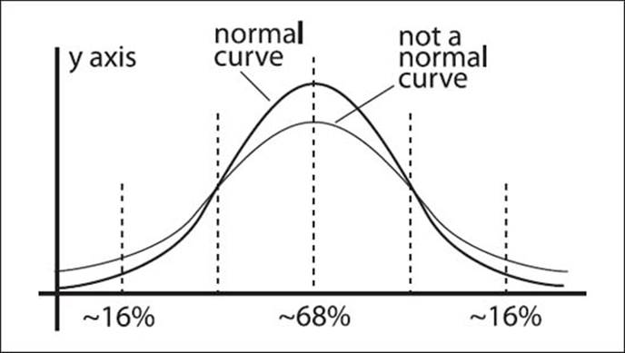
A “normal” curve has a bell shape to it into which the majority of a sampling of statistics falls within a certain average range.

What is the variance?

The variance is the average of the squares of a set’s deviations. It is used to characterize the spread among the measures of a given population. First, calculate the mean of the scores; then measure the amount that each score deviates from the mean. Finally, square that deviation (in other words, multiply it by itself, add all of them together, then divide by the total number of scores). An even easier way is to square the numbers first. (Note: Taking the square root of the variance gives the standard deviation.)

For example, take the numbers 3, 5, 8, and 9, with a mean of 6.25 (the sum of the numbers divided by the total number of numbers). To calculate the variance, determine the deviation of each number from 6.25 (3.25, 1.25, 1.75, 2.75), square each deviation (10.5625, 1.5625, 3.0625, 7.5625), then take the average 22.75/4 = 5.6875, which is the variance. An easier way to calculate the variance is to square all the numbers first (9, 25, 64, 81) and determine the mean (9 + 25 + 64 + 81 divided by 4 = 44.75). Then subtract the square of the first mean (6.25² = 39.0625)—or 44.75 - 39.0625 = 5.6875.

What is the standard deviation?

The standard deviation is considered by some to be the second most important statistic (or statistical measure) in the field; it is the measure of how much the individual observations are scattered about the mean. In general, the more widely values are spread out, the larger the standard deviation. For example, if the test results for two different exams taken by 50 people in a geology class range from 30 to 98 percent for the first exam and 78 to 95 percent for the second exam, the standard deviation is larger for the first list of exams. This spread (dispersion) of a data set is calculated by taking the square root of the variance; the notation for standard deviation is most commonly seen as follows: (or simply s), in which V(x) is the variance.

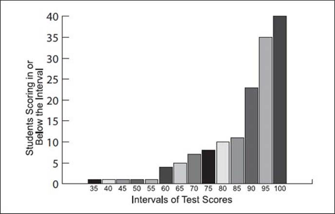
In this example of a cumulative distribution chart, all students (100 percent) fall within the maximum score of 100, while smaller numbers of students fall within each progressively lower score on a test.

What is a normal distribution?

A normal distribution is an idealized view of the world, producing the familiar, symmetrically shaped “bell-shaped curve.” It is usually based on a large set of measurements of one quantity—such as weights, test scores, or height—which are arranged by size. In a normal distribution, more than two-thirds of the measurements fall in the central region of the graph; about one-sixth of them are found on either side. Many of us are familiar with the normal distribution from standardized school test scores, as most result in a bell-shaped curve, with students hoping to at least fall in the middle of the curve.

What is a cumulative distribution?

A cumulative distribution is a plot of the number of observations that fall in or below an interval. For example, they are often used to determine where scores fall in a standardized test. For example, the x-axis (see bar graph illustration) shows the intervals of scores (such as the interval labeled 35 shows any score from 32.5 to 37.5, and so on) and the y-axis shows the number of students scoring in or below each interval. This graphically illustrates for the students (and teachers) how well they did on the test compared to other students.

What are skewness and symmetry?

Skewness is when there is asymmetry in the distribution of the sample data values. In this case, the values on one side of the distribution seem to be further from the “middle” range than values on the other side. Symmetry essentially means balance: when the data values are distributed in the same way above and below (or on both sides of) the middle of the sample.

What is a statistical test?

A statistical test is a procedure used to decide if an assertion (often called a hypothesis) about a population’s chosen quantitative feature is true or false. These tests usually entail drawing on a random sample (or simple random sample) from the chosen population, then calculating a statistic about the chosen feature. From the result, a statistician can usually determine if the hypothesis is true, false, rare, common, or something in between. Overall, for a statistical test to be valid, it is necessary to choose what statistic to use, what sample size, and what criteria to use for rejection or acceptance of the tested hypothesis.

What does the term “statistically significant” mean?

For most of us, “significant” means important; in statistics it means probably true (not due to chance) but not necessarily important. In particular, significance levels in statistics show how likely a result is due to chance. The most common level—one thought to make it good enough to believe—is 0.95, which means the finding has a 95 percent chance of being true.

This can also be misleading, however. No statistical report will indicate a 95 percent, or 0.95, in its answer, but it will show the number 0.05. Thus, statisticians say the results in a “backward” manner: they say that a finding has a 5 percent chance of not being true. To find the significance level, all one has to do is subtract the number shown from 1. For example, a value of 0.05 means that there is a 95 percent (1 - .05 5 0.95) chance of it being true; for a value of 0.01, there is a 99 percent chance (1 - 0.01 5 0.99) of it being true; and so on.

How is statistical data presented?

There are many ways to present statistical data, all of which involve graphical means to translate the results of statistical tests. A histogram is a graphical representation of a distribution function using rectangles. It is also most often constructed from a frequency table (see below). The widths of the rectangles usually indicate the intervals into which the range of observed values are divided; the heights of the rectangles indicate the number of observations that occur in each interval. The shapes of histograms vary depending on the chosen size of the intervals.

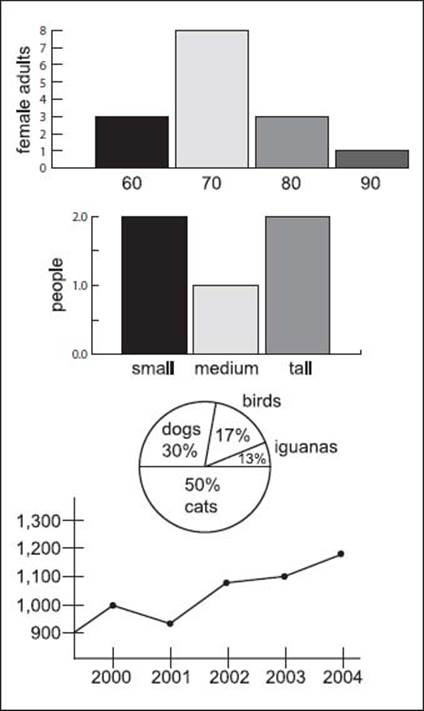
Here are four different types of charts used in statistics (from top to bottom): a histogram, a bar graph, a pie chart, and a line graph (statistics are not based on actual data here).

Bar graphs are similar to histograms, but with the columns separated by each other by small distances. They are commonly used for qualitative variables. A pie chart is another way to represent data graphically. In this case, it is a circle divided into segments, or “pie” wedges. Each segment represents not only a certain category, but its proportion to the total set of data. Another type of graph is the line graph, which is similar to those seen in geometry: a representation of the data from connected point to connected point. They are one of the most common graphs seen for simple statistical data collection.

What is a percent?

A percent (using the symbol %) is the ratio of one number to another. Percents are quantitative terms in which n percent of a number is n one-hundredths of the number; they are usually expressed as the equivalent ratio of some number to the number 100. For example, the ratio of 25 to 50 means the number 25 is 50 percent of 50. They are not true numbers; thus, percents can’t be used in calculations, such as addition or multiplication. But operations can be conducted with percents when they are translated into ratios and fractions, such as 25 percent is equal to 0.25 or 1/4.

What is a frequency table?

A frequency table is a way of summarizing data. In particular, it is a way of displaying how entities (such as scores, number of people, etc.) are divided into intervals, and of counting the number of entities in each interval. The result shows the actual number of entities, and even the percentage of entities in each interval. For example, if we survey the number of people working in the 10 offices in a building, the data set might look like the following:

Another way to present this data is to note how many offices had 1, 2, 3, or 4 people working in them. This is known as finding the frequencies of each of the data values. An example of such a frequency table would be as follows:

This is a compact way of showing how the data values are distributed between the various number of people. It allows us to see, at a glance, the most “popular” number (also called the “modal class”) of people working in an office for this building’s 10 offices—in this case, a one-person office. Such data can further be visualized with the use of bar charts, histograms, or pie charts.

There are even more ways to see the data from this frequency table. We can also illustrate this chart in terms of percent. In particular, we can say that 40 percent of the offices contain 1 person, 20 percent have 2 people, 20 percent have 3 people, and 20 percent have 4 people.

MODELING AND SIMULATION

What is a mathematical model?

Mathematical models are a way of analyzing systems by using equations (mathematical language) to determine how the system changes from one state to the next (usually using differential equations) and/or how one variable depends on the value or state of other variables. Simply put (although working through the equations is not always simple), the process of mathematical modeling includes the input of data and information, a way of processing the information, and an output of results.

A mathematical model can describe the behavior of many systems, including systems in the fields of biology, economics, social science, electrical and mechanical engineering, and thermodynamics. For example, modeling is usually used in the sciences to better understand physical phenomena; each phenomenon is translated into a set of equations that describe it. But don’t think that all the results of models are indicative of the real world. Because it is virtually impossible to describe a phenomenon totally, models are considered to be merely a human construct to help us better understand our surrounding real-world systems.

What are some types of mathematical models?

Mathematical models are commonly broken down into numerical or analytical models. Numerical models are those that use some type of numerical timing procedures to figure out a model’s behavior over time. The solution is usually represented by a table or graph. An analytical model usually has a closed solution. In other words, the solution to the equations used to describe changes in the system can be expressed as a mathematical analytic function. Mathematical models can also be divided in other ways. For example, some models are considered deterministic (or a model that always performs the same way for a given set of initial conditions) or stochastic (or a model in which randomness is present).

What are some basic steps to building a mathematical model?

Just like building a physical structure, there are basic steps to building a mathematical model. The first steps are to simplify the assumptions, or to clearly state those assumptions on which the model will be based, including an understandable account of the relationships among the quantities to be analyzed. Second is to describe all the variables and parameters to be used in the model, and identify the initial conditions of the model. Finally, use step one’s assumptions and step two’s parameters and variables to derive mathematical equations.

What is a common example of mathematical modeling?

One of the most common examples of a mathematical model has to do with the growth of populations—human, animal, or otherwise. In the sciences, this type of mathematical modeling often leads to intelligent hypotheses about the future and past of a population—from a possible population explosion to even extinctions. (For more information about the use of mathematical modeling in the sciences, see “Math in the Natural Sciences.”)

What does a priori refer to in mathematical modeling?

The term a priori refers to the amount of information available in a system. Based on the amount of a priori information, mathematical modeling problems are often classified into white-box (a system in which all necessary information is available) or black-box (a system in which there is no a priori information available) models. Practically all systems are somewhere between the white-box and black-box models; thus, this concept only works as an intuitive guide on how to approach a mathematical problem.

Many different types of data, including air pressure, temperature, humidity, and so on, must be taken into account when constructing computer models of hurricanes.

Can a mathematical model be too complex?

Yes, mathematical models can be too complex for a number of reasons. For example, if we wanted to model the development of a hurricane, we would take data from a forming storm—water vapor, pressure, temperature, and so on—and incorporate it into our model. In this way, we would try to develop as close to a white-box model of the hurricane system as possible.

But in reality a collection of such a huge amount of data—not to mention the computational cost—would effectively inhibit the use of such a weather model. There is also uncertainty because the development of a hurricane is an overly complex system, mainly because each separate part of a hurricane and its development causes some amount of variance in the model. For example, not only would we have to know about the details of the hurricane’s development, but other factors would come into play, such as the ocean-interaction variables that contribute to the hurricane, variability of solar radiation, and even how periodic events such as El Niño—a periodic warming of the waters off the South America coast—affect the hurricane. Thus, meteorologists usually use some approximations to make the mathematical model more manageable, which is also why we still can’t predict where and how much rain, wind, and tornadoes will occur during a hurricane.

How do simulators work?

Simulators use an interactive, physical device to simulate reality. For example, space shuttle simulators were used to help astronauts understand the intricacies and various scenarios associated with flying the shuttle; people can even improve their driving skills using driving simulators. But how do simulators work in terms of mathematics?

One way of seeing how this works is with an airplane flight simulator. Although there are different types—ranging from full cockpit to full motion simulators—they have the same purpose: to make the person “flying” the simulator feel as if he or she is really controlling an airplane. When a person sits in the cockpit, he or she sees a virtual world projected onto a screen—what it would look like outside a real plane’s cockpit. As the pilot “flies” by moving the instruments, the actions get translated to a computer hooked to the simulator; from there, each component of the process is translated using physics-based equations that describe the relationship between the input and output of the actions. Not only do the instruments respond in kind, but often, if the simulator is hooked to hydraulic mounts, movements will also be fed by computer into the simulator. Thus, the pilot will truly feel as if he or she is flying—all thanks to mathematical equations translated by the computer and into the simulator.

How can the accuracy of a mathematical model be determined?

There is usually one good way to determine the accuracy of a mathematical model: Once a set of equations has been built and solved, if the data generated by the equations agree (or come close to) the real data collected from the system, then we can determine its accuracy. In fact, the set of equations and models are only “valid” as long as the two sets of data are close. If a model result leads to conclusions that are not close to the real-world scenario, then the equations are further modified to correct for the discrepancies as much as possible.

For example, in weather prognostication, meteorologists use various numerical models to make long-term predictions of weather systems (for more information about models and weather prediction, see “Math in the Natural Sciences”). It is interesting to see how meteorologists use a combination of several of the weather models to forecast the weather in certain spots around the United States and the world— mainly because no weather forecasting model has all the right answers. Every day, researchers are tweaking their respective weather models (based on more collected data) in hopes of eventually understanding our weather a bit better.

What is a simulation?

A simulation is an imitation of some real event or device. It is often used interchangeably with the word modeling (as in modeling of natural systems). A simulation tries to represent certain features (or behaviors) of a complex physical system based on the underlying computational models of the phenomenon, environment, or experience.

Simulations are used to understand the operation of real-world, practical systems; for instance, the modeling of natural systems such as the human body. They can be used to simulate a certain type of technology, such as a new type of airplane, or model an engineering concern, such as the stability of a building during an earthquake.

OTHER AREAS OF APPLIED MATHEMATICS

What is numerical analysis?

Numerical analysis is a branch of applied mathematics that studies certain specialized techniques for solving mathematical problems; in particular, it is the study of algorithms that use numerical approximation for mathematical analysis problems. In general, it employs mathematical axioms, theorems, and proofs, and often uses empirical results to further analyze or examine new methods. Characteristics of numerical analysis methods include accuracy (the numerical approximation should be as accurate as possible); robustness (the algorithm should be able to solve many problems and should relate to the user when the results are inaccurate); and speed (the faster the computation, the better the method).

What are some areas that numerical analysis addresses?

Areas addressed by numerical analysis include computing the values of functions, solving equations, optimizing functions, evaluating integrals, and solving for differential equations. (For more about these areas, see “Mathematical Analysis.”)

How does the Monte Carlo method work?

The Monte Carlo method has been used for centuries, but it was not truly thought of as a “viable” mathematical technique until around the first half of the 20th century. Some people say it was named after the city in the Monaco principality because of the simple random number generator of roulette played in the Monaco casinos; others say the method’s creator was honoring a relative having a propensity toward gambling.

It’s known that Italian physicist Enrico Fermi (1901–1954) not only used the method to calculate neutron diffusion, but invented the Fermiac, a Monte Carlo mechanical device to determine the criticality in nuclear reactors. Further foundations of the method were laid down in the 1940s by Hungarian mathematician John von Neumann (1903–1957), along with Polish mathematician Stanislaw Ulam (1909–1984); and Nicholas Metropolis would go on to invent the computer chess program MANIAC I—the first to beat a human player—based on von Neumann’s work. Simply put, the Monte Carlo method gives approximate numerical solutions to a number of problems that are too difficult to solve analytically by performing specific statistical sampling experiments. Although forms of the method have been known for a while, it was initially developed for numerical integrations in statistical physics problems during the early days of electronic computing.

But there is more to the Monte Carlo method than meets the computation. First, it’s actually thought of now as a true numerical method that addresses some of the most complex mathematical applications. The list of applications seems endless, including cancer therapy, Dow-Jones forecasts, and stellar evolution. Second, there is more than one Monte Carlo method. For example, one method, called the Markov chain Monte Carlo method, has played a critical role in such diverse fields as physics, statistics, computer science, and structural biology. And the list of applications is long, especially in its usefulness and power for all types of prediction.

Italian physicist Enrico Fermi used the Monte Carlo method to calculate neutron diffusion and to invent a device that determined criticality in nuclear reactors.

What is operations research?

Operations research, more commonly called optimization theory, is a form of applied mathematics designed to determine the most efficient way of doing something by using mathematical models, statistics, and algorithms in the decision-making process. It is a branch of mathematics that entails the many diverse areas of optimization and minimization, including the calculus of variations, control theory, decision theory, game theory, linear programming, and many others. Operations research is most often used to analyze complex, real-world systems, stressing the improvement in or optimization of performance.

What is some of the history behind operations research?

In the United Kingdom, operations research is known as operational research; other English-speaking countries most often use the term “operations research” (OR). The idea of operations research started during World War II, when military planners in the United States and United Kingdom were searching for ways to make better decisions in the fields of logistics and training schedules. Unlike its origins, today’s applications in operations research have little to do with its traditional sense. In other words, it’s not applied to the battlefield, but to logistical, scheduling, and other such decisions in industry.

What are some applications of operations research?

Applications of operations research span a wide variety of fields, especially with regard to reducing costs or increasing efficiency. The following lists just a few examples: constructing a telecommunications network at low cost and top efficiency, especially when under high demand or after being damaged; determining routes of school buses so fewer vehicles are needed; and designing a computer chip that will reduce manufacturing time.

What is optimization?

Optimization problems deal with the point at which a given function is maximized (or minimized). It is divided into several subfields, depending on the form of the objective function and the constraints that the maximized point often has to satisfy.

What is information theory?

Information theory is a branch of the mathematical theory of probability and statistics, allowing it to quantify concepts of information. It was formulated primarily by American scientist Claude E. Shannon (1916-2001; who was also called “the father of information theory”) to explain the aspects and problems inherent in information and communication. In particular, it involves efficient and accurate storage, transmission, and representation of information, such as the engineering requirements—and limitations—of communication systems. (Note: Information theory has nothing to do with library and information science or with information technology.)

In information theory, the term “information” is not used in the traditional sense. Here it is used to mean a measure of the freedom of choice with which a message is selected from the set of all possible messages. Because it is possible for a string of nonsense words and a meaningful sentence to be equivalent with respect to information content, “information” in this sense takes on a different meaning.

What is game theory?

As the words imply, game theory has to do with the mathematics and logic used in the analysis of games—or the situations that involve groups with conflicting interests. Another way to look at a game is as a conflict that involves gains and losses between two or more opponents who all follow a set of formal rules.

In particular, game theorists study the predicted and actual behavior of individuals in specific games, as well as the optimal strategies used in the games. Thus, the principles of game theory can be applied to games such as cards, checkers, and chess; or, they can be applied to real-world problems in economics, politics, psychology, and even warfare. For example, game theory is used to determine optimal policy choices of presidential candidates, or even to analyze major league baseball salary negotiations.